View connectedness of two factors in a dataframe using a levelplot
Source:R/functions.R
con_view.RdIf there is replication for the treatment combination cells in a two-way table, the replications are averaged together (or counted) before constructing the heatmap.
By default, rows and columns are clustered using the 'incidence' matrix of 0s and 1s.
The function checks to see if the cells in the heatmap form a connected set. If not, the data is divided into connected subsets and the subset group number is shown within each cell.
By default, missing values in the response are deleted. If no response variable is specified a constant response value of 1 is used.
Factor levels are shown along the left and bottom sides.
The number of cells in each column/row is shown along the top/right sides.
If the 2 factors are disconnected, the group membership ID is shown in each cell.
Usage
con_view(
  data,
  formula,
  fun.aggregate = mean,
  xlab = "",
  ylab = "",
  cex.num = 0.75,
  cex.x = 0.7,
  cex.y = 0.7,
  col.regions = RedGrayBlue,
  cluster = "incidence",
  dropNA = TRUE,
  ...
)
Arguments
- data
A dataframe
- formula
A formula with two (or more) factor names in the dataframe like
yield ~ f1 *f2- fun.aggregate
The function to use for aggregating data in cells. Default is mean.
- xlab
Label for x axis
- ylab
Label for y axis
- cex.num
Disjoint group number.
- cex.x
Scale factor for x axis tick labels. Default 0.7.
- cex.y
Scale factor for y axis tick labels Default 0.7.
- col.regions
Function for color regions. Default RedGrayBlue.
- cluster
If "incidence" or TRUE, cluster rows and columns by the incidence matrix. If FALSE, no clustering is performed.
- dropNA
If TRUE, observed data that are
NAwill be dropped.- ...
Other parameters passed to the levelplot() function.
Examples
require(lattice)
bar = transform(lattice::barley, env=factor(paste(site,year)))
set.seed(123)
bar <- bar[sample(1:nrow(bar), 70, replace=TRUE),]
con_view(bar, yield ~ variety * env, cex.x=1, cex.y=.3, cluster=FALSE)
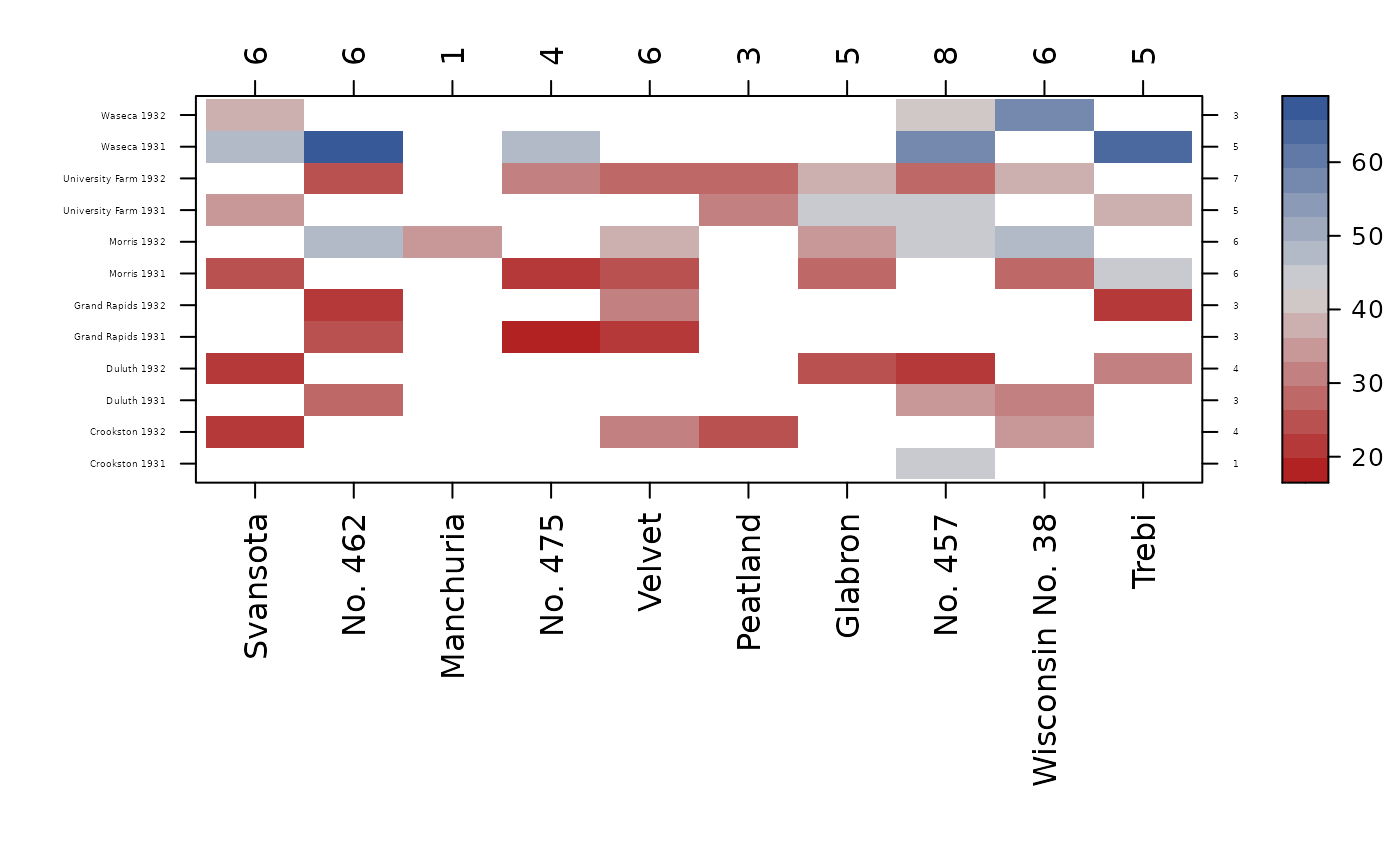 con_view(bar, ~ variety * env, cex.x=1, cex.y=.3, cluster=FALSE)
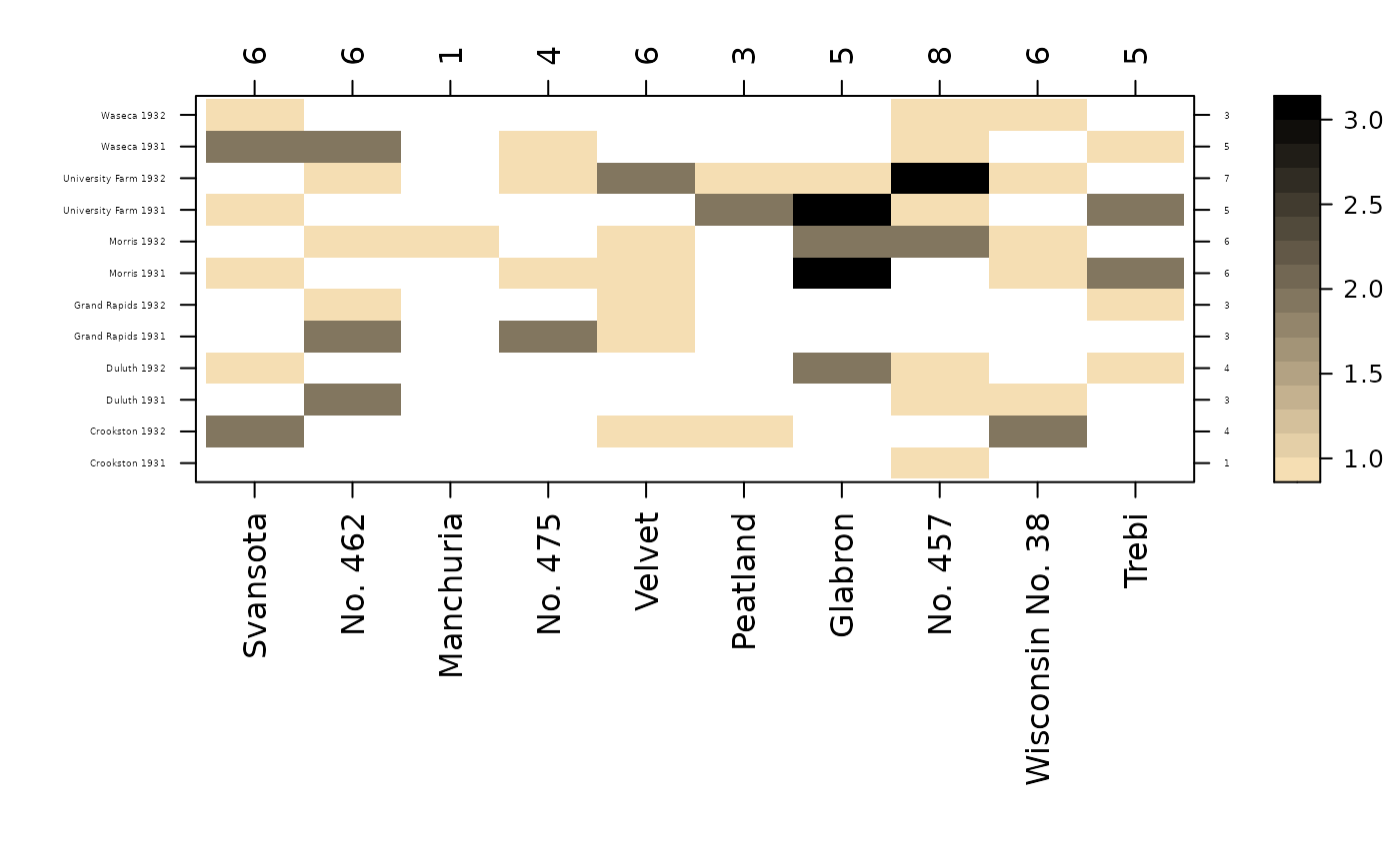 # Create a heatmap of cell counts
w2b = colorRampPalette(c('wheat','black'))
con_view(bar, yield ~ variety * env, fun.aggregate=length,
cex.x=1, cex.y=.3, col.regions=w2b, cluster=FALSE)
# Create a heatmap of cell counts
w2b = colorRampPalette(c('wheat','black'))
con_view(bar, yield ~ variety * env, fun.aggregate=length,
cex.x=1, cex.y=.3, col.regions=w2b, cluster=FALSE)
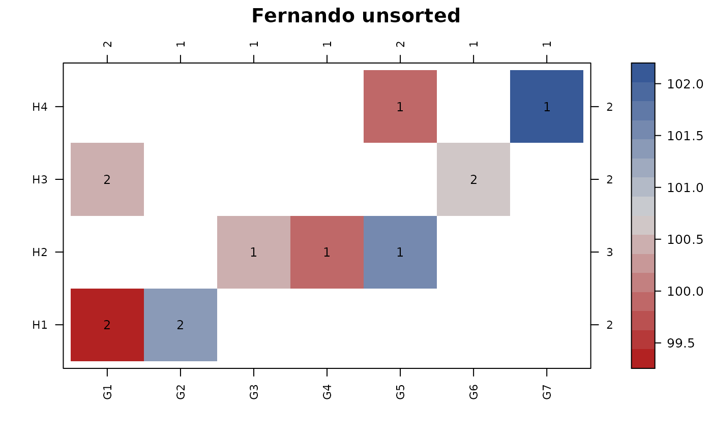
 # Example from paper by Fernando et al. (1983).
set.seed(42)
data_fernando = transform(data_fernando,
y=stats::rnorm(9, mean=100))
con_view(data_fernando, y ~ gen*herd, cluster=FALSE,
main = "Fernando unsorted")
#> Warning: There are 2 disconnected groups
# Example from paper by Fernando et al. (1983).
set.seed(42)
data_fernando = transform(data_fernando,
y=stats::rnorm(9, mean=100))
con_view(data_fernando, y ~ gen*herd, cluster=FALSE,
main = "Fernando unsorted")
#> Warning: There are 2 disconnected groups
 con_view(data_fernando, y ~ gen*herd,
main = "Fernando clustered")
#> Warning: There are 2 disconnected groups
con_view(data_fernando, y ~ gen*herd,
main = "Fernando clustered")
#> Warning: There are 2 disconnected groups
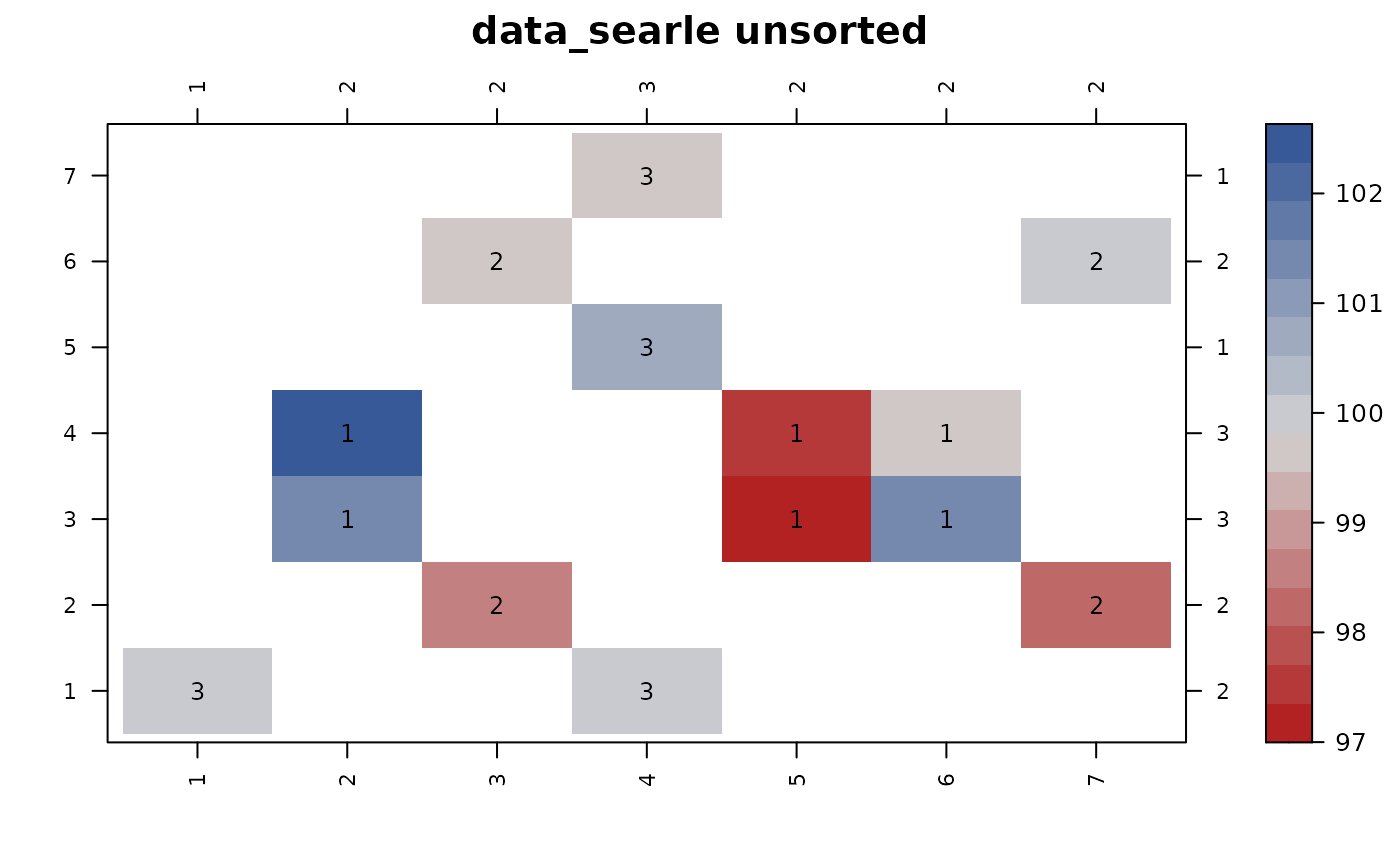 # Example from Searle (1971), Linear Models, p. 325
dat2 = transform(data_searle,
y=stats::rnorm(nrow(data_searle)) + 100)
con_view(dat2, y ~ f1*f2, cluster=FALSE, main="data_searle unsorted")
#> Warning: There are 3 disconnected groups
# Example from Searle (1971), Linear Models, p. 325
dat2 = transform(data_searle,
y=stats::rnorm(nrow(data_searle)) + 100)
con_view(dat2, y ~ f1*f2, cluster=FALSE, main="data_searle unsorted")
#> Warning: There are 3 disconnected groups
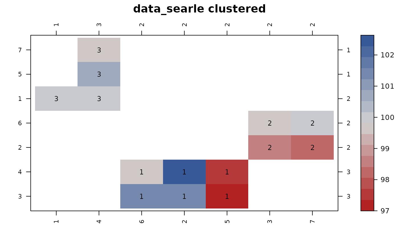 con_view(dat2, y ~ f1*f2, main="data_searle clustered")
#> Warning: There are 3 disconnected groups
con_view(dat2, y ~ f1*f2, main="data_searle clustered")
#> Warning: There are 3 disconnected groups
