Mountainplot

A mountain plot is similar to an empirical CDF, but _decreases_ from .5 down to 1, using a separate scale on the right axis.

Usage

mountainplot(x, data, ...)

mountainplotyscale.components(...)

# S3 method for class 'formula'
mountainplot(
  x,
  data = NULL,
  prepanel = "prepanel.mountainplot",
  panel = "panel.mountainplot",
  ylab = gettext("Folded Empirical CDF"),
  yscale.components = mountainplotyscale.components,
  scales = list(y = list(alternating = 3)),
  ...
)

# S3 method for class 'numeric'
mountainplot(x, data = NULL, xlab = deparse(substitute(x)), ...)

Arguments

x

Variable in the data.frame 'data'.

data

A data frame

...

Other arguments

prepanel

The prepanel function. Default "prepanel.mountainplot".

panel

The panel function. Default "panel.mountainplot".

ylab

Vertical axis label.

yscale.components

Function for drawing left and right side axes.

scales

The "scales" argument used by lattice functions.

xlab

Horizontal axis label.

Value

A lattice object

Details

Note that `mountainplotyscale.components` is not really intended to be called by the user, but is used by lattice to configure the right-axis ticks and labels.

References

K. L. Monti. (1995). Folded empirical distribution function curves-mountain plots. The American Statistician, 49, 342–345. http://www.jstor.org/stable/2684570

Xue, J. H., & Titterington, D. M. (2011). The p-folded cumulative distribution function and the mean absolute deviation from the p-quantile. Statistics & Probability Letters, 81(8), 1179-1182.

Examples

data(singer, package = "lattice")
singer <- within(singer, {
section <- voice.part
section <- gsub(" 1", "", section)
section <- gsub(" 2", "", section)
section <- factor(section)
})
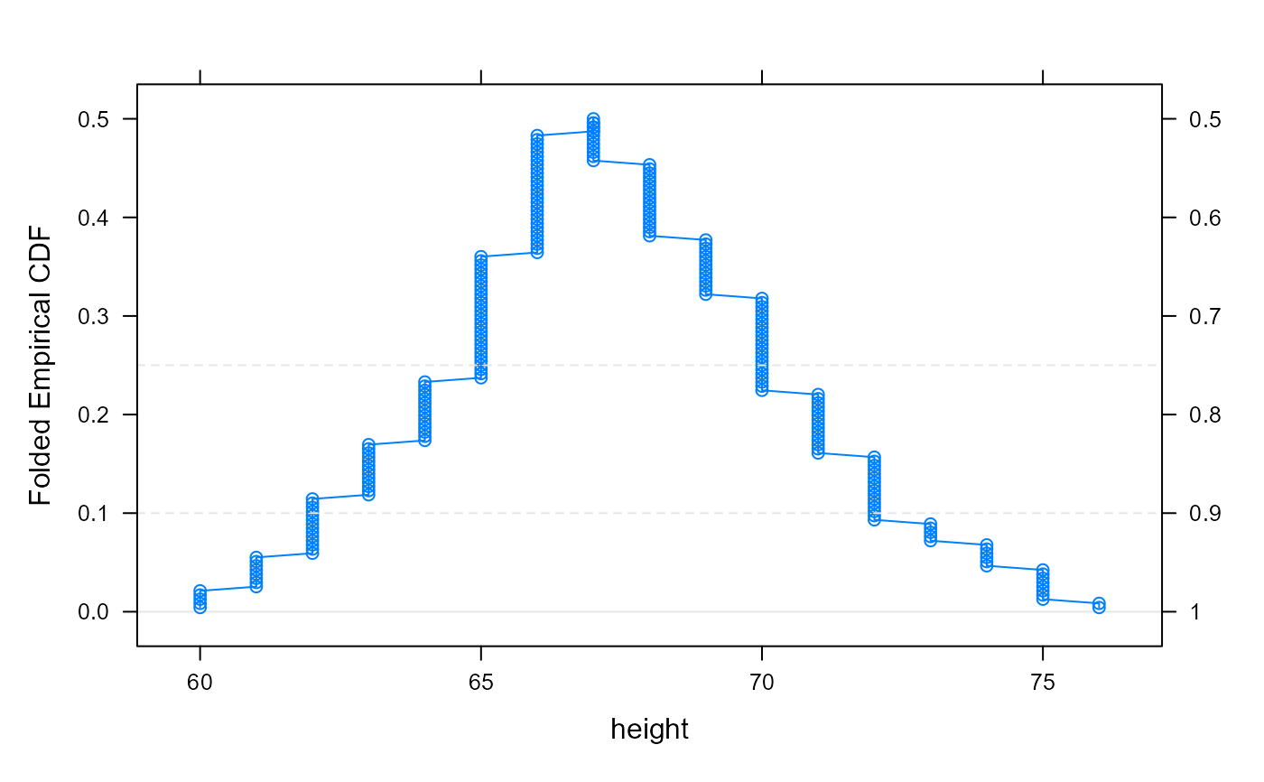
mountainplot(~height, data = singer, type='b')

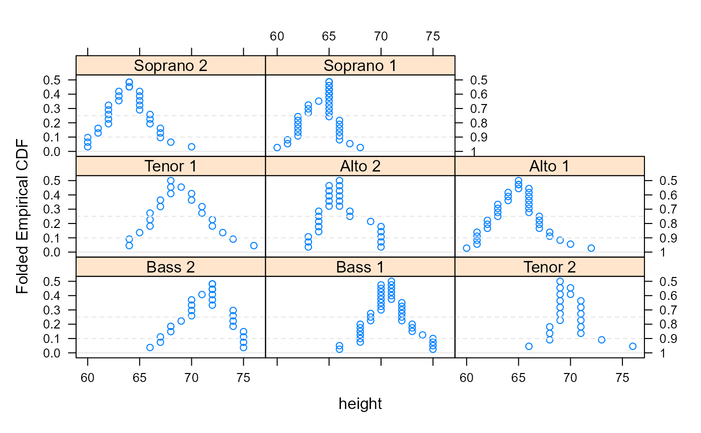
mountainplot(~height|voice.part, data = singer, type='p')

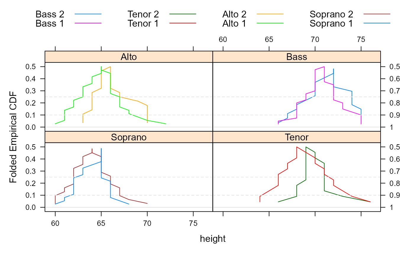
mountainplot(~height|section, data = singer, groups=voice.part, type='l',
auto.key=list(columns=4), as.table=TRUE)