Data do not always come in a format that you can readily use for analysis. Some cleaning and restructuring of data is often needed despite of the size of the dataset.

Raw data

This data was downloaded 15 Apr 2019 from TidyTuesday. The full description of the data are here: https://github.com/rfordatascience/tidytuesday/files/2343596/Hypoxia.Article.proof.pdf.

Briefly, the data:

X1 - Dummy. Row number.
Altitude - Altitude.
Air press - Air pressure.
ppO2 - Part of pressure related to oxygen.
Alv pO2 - Pressure of O2 in lungs.
% sat O2 - Percentage of hemoglobin molecules with O2.
Alv pCO2 - Pressure of carbion dioxide in lungs.
Alv pO2 with O2=100% - Maximum O2 pressure in lungs without mask.
% sat O2_1 - Best saturation possible without mask.
Alv pCO2_1 - Pressure of CO2 in lungs with 100% O2.

Before looking at the data, make sure that we do not missinterpret any entry when reading the file. For csv and txt files it is safe to read each columns as text. Also, it is good practice to read only the first few rows (5 in this case) of data for this purpose.

library(tidyverse)
datfile <- system.file("messydata", "hypoxia.csv", package="untidydata2")
read_csv(datfile, col_types = cols(.default = "c"), n_max = 5) %>%
  knitr::kable()

X1	Altitude	Air press	ppO2	Alv pO2	% sat O2	Alv pCO2	Alv pO2 with O2=100%	% sat O2_1	Alv pCO2_1
1	Ft/m	mmHg	Air=21%	mmHg on air	>90% desired	>35 best	NA	100% O2	100% O2
2	Sea level	760	159	104	97	40	673	100	40
3	10k/3k	523	110	67	90	36	436	100	40
4	20k/6.1k	349	73	40	73	24	262	100	40
5	30k/9.1k	226	47	18	24	24	139	99	40

Problems

There are several problems that one can note at first glance.

variable description is included in the first row
column names contain spaces and symbols
first column is redandant and inaccurate (first row is assigned 1, even though it does not represent an observation)
variable ‘Altitude’ contains two values in different units and non-numeric record (‘Sea level’)
last three variables are the same as previous 3 columns, but at different oxygen content (percentge)

Tidying the data

First we need to fix the variable names. The best way is to manually define each variable name after reading the data without column names. Since the last 6 columns represent the same variable measured at different oxygen levels, we will incorporate this piece of info in the variable names (and use later when reshaping the data).

data <- read_csv(datfile, 
                 col_types = cols(.default = "?"), 
                 col_names = FALSE,
                 skip = 2) %>% 
  # remove first cloumn 
  select(-1) %>% 
  # set names of variables 
  set_names(c('altitude', 'air_pressure', 'ppO2', 
              'alveoli_pO2-21', 'sturation_O2-21', 'alveoli_pCO2-21',
              'alveoli_pO2-100', 'sturation_O2-100', 'alveoli_pCO2-100'))

After reading the data we will address remaining problems listed as follow:

tidy_data <- data %>%
  # set 'Sea level' as 0 ft and 0 m in format matching the other records in altitude
  mutate(altitude = ifelse(altitude == 'Sea level', '0k/0k', altitude)) %>%
  # split altitude data into columns corresponding to each unit of measurement
  separate(altitude, into = c('altitude_ft', 'altitude_m'), sep = '/') %>%
  # convert altitude into numeric data by taking into account k
  mutate_at(vars(starts_with('altitude')), parse_number) %>%
  mutate_at(vars(starts_with('altitude')), funs(. * 1000)) %>%
  # handle last 6 columns
  gather(key, value, 5:10) %>%
  # extract oxygen level (that was incorporated into the variable name earlier)
  separate(key, into = c('variable', 'O2'), sep = '-', convert = TRUE) %>%
  spread(variable, value) %>%
  arrange(O2, altitude_ft)

## Warning: funs() is soft deprecated as of dplyr 0.8.0
## Please use a list of either functions or lambdas: 
## 
##   # Simple named list: 
##   list(mean = mean, median = median)
## 
##   # Auto named with `tibble::lst()`: 
##   tibble::lst(mean, median)
## 
##   # Using lambdas
##   list(~ mean(., trim = .2), ~ median(., na.rm = TRUE))
## This warning is displayed once per session.

knitr::kable(tidy_data)

altitude_ft	altitude_m	air_pressure	ppO2	O2	alveoli_pCO2	alveoli_pO2	sturation_O2
0	0	760	159	21	40	104	97
10000	3000	523	110	21	36	67	90
20000	6100	349	73	21	24	40	73
30000	9100	226	47	21	24	18	24
40000	12000	141	29	21	NaN	NaN	NaN
50000	15200	87	18	21	NaN	NaN	NaN
0	0	760	159	100	40	673	100
10000	3000	523	110	100	40	436	100
20000	6100	349	73	100	40	262	100
30000	9100	226	47	100	40	139	99
40000	12000	141	29	100	36	58	84
50000	15200	87	18	100	24	16	15

Plot

We can plot some data.

tidy_data %>%
  mutate(O2 = factor(O2, levels = c(21, 100), labels = c('21%', '100%'))) %>%
  ggplot(aes(x = alveoli_pO2, y = altitude_m)) +
  geom_point(aes(colour = O2), na.rm = TRUE) +
  theme_light()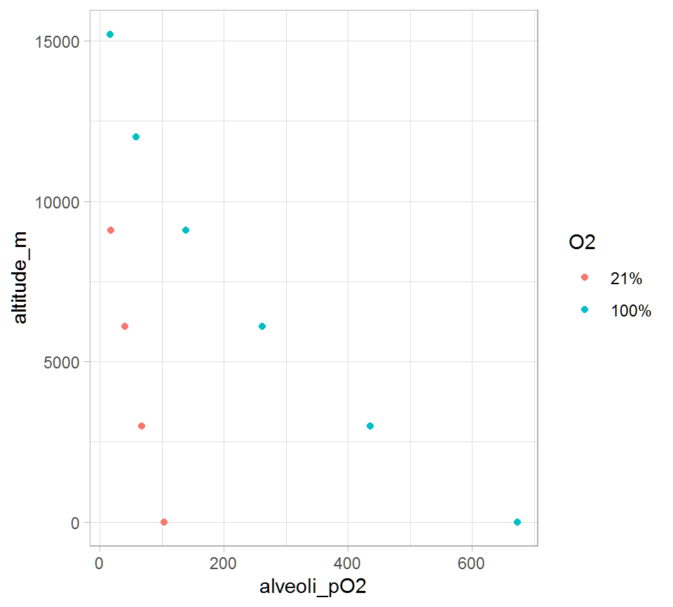

As an airplane pilot flies at higher altitudes, the pressure of oxygen in the lungs decreases.

Hypoxia Data

Giorgi Chighladze

2019-09-13

Raw data

Problems

Tidying the data

Plot

Contents