Raw data

This vignette is about working with an untidy spreadsheet of simulated sales data for a fictitious company with multiple locations in Indiana. The document presents several challenges we often encounter with real spreadsheets, including:

Separate sheets (tabs) for groups in the data (in this case year)
Multiple header rows, including one with “merged cells”
Repeated headers within the same sheet
Number of columns varies by sheet

The document contains 10 sheets (tabs), so coding them one-by-one isn’t very appealing. We’ll want to automate processing the sheets.

Manually process a representative sheet

Before we create an automated solution, let’s start by manually processing a representative sheet so we can figure out what we need to automate.

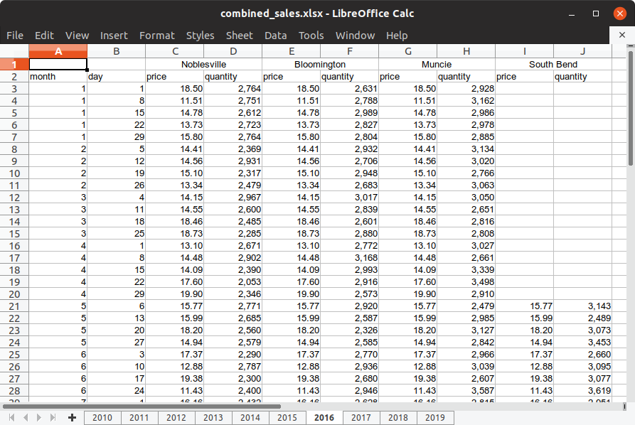
Open the document in your favorite spreadsheet software and you’ll see that the first few sheets contain data for just one location, Noblesville. Later sheets contain data for more than one location. Sheet 7 (for 2016) looks like a good one to work with because it has data for multiple locations.

Notice that the location names are in cells that have been merged and centered, and there are price and quantity columns for each of the locations. Also notice that data for the last location, South Bend, is missing for the first several rows.

Let’s start by loading the tidyverse and readxl packages and setting file_name to the path to the spreadsheet. Since the spreadsheet is part of the untidydata2 package, we use system.file to return a path to the spreadsheet.

library(tidyverse)

## -- Attaching packages ---------------------------------- tidyverse 1.2.1 --

## v ggplot2 3.2.1     v purrr   0.3.2
## v tibble  2.1.3     v dplyr   0.8.3
## v tidyr   0.8.3     v stringr 1.4.0
## v readr   1.3.1     v forcats 0.4.0

## -- Conflicts ------------------------------------- tidyverse_conflicts() --
## x dplyr::filter() masks stats::filter()
## x dplyr::lag()    masks stats::lag()

library(readxl)

file_name <- system.file("messydata", "combined_sales.xlsx", package="untidydata2")

First, let’s get a list of locations contained in sheet for 2016 using readxl::read_excel. We can read just the first row by setting n_max = 0 and then passing the result to names.

read_excel(file_name, sheet = "2016", n_max = 0) %>%
  names()

## [1] "Noblesville" "...2"        "Bloomington" "...4"        "Muncie"     
## [6] "...6"        "South Bend"

The merged cells are coming back with names of “…2”, “…4”, etc. We can remove them from the list with stringr::str_subset and a regular expressing that matches “…” at the beginning of a string.

locations <- read_excel(file_name, sheet = "2016", n_max = 0) %>%
  names() %>%
  str_subset("^\\.{3}", negate = TRUE)

locations

## [1] "Noblesville" "Bloomington" "Muncie"      "South Bend"

Now we have a character vector of locations for the 2016 sheet. Let’s read the rest of the data from the 2016 sheet, skipping the first row this time.

read_excel(file_name, sheet = "2016", skip = 1)

## # A tibble: 53 x 10
##    month   day price...3 quantity...4 price...5 quantity...6 price...7
##    <dbl> <dbl>     <dbl>        <dbl>     <dbl>        <dbl>     <dbl>
##  1     1     1      18.5        2764.      18.5        2631.      18.5
##  2     1     8      11.5        2751.      11.5        2788.      11.5
##  3     1    15      14.8        2612.      14.8        2989.      14.8
##  4     1    22      13.7        2723.      13.7        2827.      13.7
##  5     1    29      15.8        2764.      15.8        2804.      15.8
##  6     2     5      14.4        2369.      14.4        2932.      14.4
##  7     2    12      14.6        2931.      14.6        2706.      14.6
##  8     2    19      15.1        2317.      15.1        2948.      15.1
##  9     2    26      13.3        2479.      13.3        2683.      13.3
## 10     3     4      14.1        2967.      14.1        3017.      14.1
## # ... with 43 more rows, and 3 more variables: quantity...8 <dbl>,
## #   price...9 <dbl>, quantity...10 <dbl>

We’re making progress but we need to do something to associate the price... and quantity... variables with their correct locations. Later we will want to have a separate variable for location, but for now let’s rename our price and quantity variables to price_Noblesville, quantity_Noblesville, price_Bloomington, quantity_Bloomington, etc.

Notice that price...3 and quantity...4 correspond to the first location, price...5 and quantity...6 correspond to the second location, etc. Let’s write a function to give us the corresponding location index for each value 3, 4, 5, 6, etc.

loc_index <- function(n) {
  floor((n-1)/2)
}

Now let’s verify that this works.

loc_index(3:10)

## [1] 1 1 2 2 3 3 4 4

Yes it does.

Now we can write a function to calculate a new name for each column we want to rename.

new_name <- function(columns) {
  num <- as.integer(str_extract(columns, "\\d+"))
  location <- locations[loc_index(num)]
  str_replace(columns, paste0("...", num), paste0("_", location))
}

And let’s verify that this works.

new_name(c("price...3", "quantity...4", "price...5", "quantity...6"))

## [1] "price_Noblesville"    "quantity_Noblesville" "price_Bloomington"   
## [4] "quantity_Bloomington"

Okay. Now we’re ready to read the spreadsheet and rename the columns.

data_2016 <- read_excel(file_name, sheet = "2016", skip = 1) %>%
  rename_at(vars(contains("...")), new_name)

data_2016

## # A tibble: 53 x 10
##    month   day price_Noblesvil~ quantity_Nobles~ price_Bloomingt~
##    <dbl> <dbl>            <dbl>            <dbl>            <dbl>
##  1     1     1             18.5            2764.             18.5
##  2     1     8             11.5            2751.             11.5
##  3     1    15             14.8            2612.             14.8
##  4     1    22             13.7            2723.             13.7
##  5     1    29             15.8            2764.             15.8
##  6     2     5             14.4            2369.             14.4
##  7     2    12             14.6            2931.             14.6
##  8     2    19             15.1            2317.             15.1
##  9     2    26             13.3            2479.             13.3
## 10     3     4             14.1            2967.             14.1
## # ... with 43 more rows, and 5 more variables: quantity_Bloomington <dbl>,
## #   price_Muncie <dbl>, quantity_Muncie <dbl>, `price_South Bend` <dbl>,
## #   `quantity_South Bend` <dbl>

The trickiest part of tidying this data

Finally, let’s extract location, price, and quantity variables. This is the trickiest part of tidying this data because it involves gathering multiple variables and then spreading them again. We also add the year and order the variables.

data_2016 %>%
  gather(-month, -day, key = "label", value = "value") %>%
  separate(label, into = c("type", "location"), sep = "_") %>%
  spread(key = "type", value = "value") %>%
  filter(!is.na(price) | !is.na(quantity)) %>%
  mutate(year = 2016) %>%
  select(year, month, day, location, price, quantity)

## # A tibble: 194 x 6
##     year month   day location    price quantity
##    <dbl> <dbl> <dbl> <chr>       <dbl>    <dbl>
##  1  2016     1     1 Bloomington  18.5    2631.
##  2  2016     1     1 Muncie       18.5    2928.
##  3  2016     1     1 Noblesville  18.5    2764.
##  4  2016     1     8 Bloomington  11.5    2788.
##  5  2016     1     8 Muncie       11.5    3162.
##  6  2016     1     8 Noblesville  11.5    2751.
##  7  2016     1    15 Bloomington  14.8    2989.
##  8  2016     1    15 Muncie       14.8    2986.
##  9  2016     1    15 Noblesville  14.8    2612.
## 10  2016     1    22 Bloomington  13.7    2827.
## # ... with 184 more rows

Whoa, there is a lot going on there! Let’s do that again and look at the intermediate results.

One more time with intermediate results

First we gather the location/price/quantity columns into label and value variables.

step1 <- data_2016 %>%
  gather(-month, -day, key = "label", value = "value")
head(step1)

## # A tibble: 6 x 4
##   month   day label             value
##   <dbl> <dbl> <chr>             <dbl>
## 1     1     1 price_Noblesville  18.5
## 2     1     8 price_Noblesville  11.5
## 3     1    15 price_Noblesville  14.8
## 4     1    22 price_Noblesville  13.7
## 5     1    29 price_Noblesville  15.8
## 6     2     5 price_Noblesville  14.4

tail(step1)

## # A tibble: 6 x 4
##   month   day label               value
##   <dbl> <dbl> <chr>               <dbl>
## 1    11    25 quantity_South Bend 3038.
## 2    12     2 quantity_South Bend 3188.
## 3    12     9 quantity_South Bend 3265.
## 4    12    16 quantity_South Bend 3487.
## 5    12    23 quantity_South Bend 2849.
## 6    12    30 quantity_South Bend 3050.

Then we can separate location into its own variable, while maintaining a type variable to distinguish price and quantity.

step2 <- step1 %>%
  separate(label, into = c("type", "location"), sep = "_")
head(step2)

## # A tibble: 6 x 5
##   month   day type  location    value
##   <dbl> <dbl> <chr> <chr>       <dbl>
## 1     1     1 price Noblesville  18.5
## 2     1     8 price Noblesville  11.5
## 3     1    15 price Noblesville  14.8
## 4     1    22 price Noblesville  13.7
## 5     1    29 price Noblesville  15.8
## 6     2     5 price Noblesville  14.4

tail(step2)

## # A tibble: 6 x 5
##   month   day type     location   value
##   <dbl> <dbl> <chr>    <chr>      <dbl>
## 1    11    25 quantity South Bend 3038.
## 2    12     2 quantity South Bend 3188.
## 3    12     9 quantity South Bend 3265.
## 4    12    16 quantity South Bend 3487.
## 5    12    23 quantity South Bend 2849.
## 6    12    30 quantity South Bend 3050.

Now we can move price and quantity into their own variables using tidyr::spread.

step3 <- step2 %>%
  spread(key = "type", value = "value")
step3

## # A tibble: 212 x 5
##    month   day location    price quantity
##    <dbl> <dbl> <chr>       <dbl>    <dbl>
##  1     1     1 Bloomington  18.5    2631.
##  2     1     1 Muncie       18.5    2928.
##  3     1     1 Noblesville  18.5    2764.
##  4     1     1 South Bend   NA        NA 
##  5     1     8 Bloomington  11.5    2788.
##  6     1     8 Muncie       11.5    3162.
##  7     1     8 Noblesville  11.5    2751.
##  8     1     8 South Bend   NA        NA 
##  9     1    15 Bloomington  14.8    2989.
## 10     1    15 Muncie       14.8    2986.
## # ... with 202 more rows

Finally, we filter out NA values, add the year, and reorder the variables.

step3 %>%
  filter(!is.na(price) | !is.na(quantity)) %>%
  mutate(year = 2016) %>%
  select(year, month, day, location, price, quantity)

## # A tibble: 194 x 6
##     year month   day location    price quantity
##    <dbl> <dbl> <dbl> <chr>       <dbl>    <dbl>
##  1  2016     1     1 Bloomington  18.5    2631.
##  2  2016     1     1 Muncie       18.5    2928.
##  3  2016     1     1 Noblesville  18.5    2764.
##  4  2016     1     8 Bloomington  11.5    2788.
##  5  2016     1     8 Muncie       11.5    3162.
##  6  2016     1     8 Noblesville  11.5    2751.
##  7  2016     1    15 Bloomington  14.8    2989.
##  8  2016     1    15 Muncie       14.8    2986.
##  9  2016     1    15 Noblesville  14.8    2612.
## 10  2016     1    22 Bloomington  13.7    2827.
## # ... with 184 more rows

This looks good, but it’s just one sheet. Now let’s write some code to process the whole spreadsheet document.

A function to read any specified sheet from the document

Here is a function that combines everything we’ve done above to read any specified sheet from the document. It also handles the simpler special case when a sheet contains only a single location.

read_sheet <- function(file_name, sheet) {
  locations <- read_excel(file_name, sheet = sheet, n_max = 0) %>%
    names() %>%
    str_subset("^\\.{3}", negate = TRUE)

  df <- read_excel(file_name, sheet = sheet, skip = 1)
  
  if (length(locations) == 1) {
    df <- df %>%
      mutate(location = locations[1])
  } else {
    loc_index <- function(n) {
      floor((n-1)/2)
    }
    
    new_name <- function(columns) {
      num <- as.integer(str_extract(columns, "\\d+"))
      location <- locations[loc_index(num)]
      str_replace(columns, paste0("...", num), paste0("_", location))
    }
    
    df <- df %>%
      rename_at(vars(contains("...")), new_name) %>%
      gather(-month, -day, key = "label", value = "value") %>%
      separate(label, into = c("type", "location"), sep = "_") %>%
      spread(key = "type", value = "value")
  }
  
  df <- df %>%
    filter(!is.na(price) | !is.na(quantity)) %>%
    mutate(year = as.integer(sheet)) %>%
    select(year, month, day, location, price, quantity)

  df
}

read_sheet(file_name, "2016")

## # A tibble: 194 x 6
##     year month   day location    price quantity
##    <int> <dbl> <dbl> <chr>       <dbl>    <dbl>
##  1  2016     1     1 Bloomington  18.5    2631.
##  2  2016     1     1 Muncie       18.5    2928.
##  3  2016     1     1 Noblesville  18.5    2764.
##  4  2016     1     8 Bloomington  11.5    2788.
##  5  2016     1     8 Muncie       11.5    3162.
##  6  2016     1     8 Noblesville  11.5    2751.
##  7  2016     1    15 Bloomington  14.8    2989.
##  8  2016     1    15 Muncie       14.8    2986.
##  9  2016     1    15 Noblesville  14.8    2612.
## 10  2016     1    22 Bloomington  13.7    2827.
## # ... with 184 more rows

The hard part is done. Now let’s read and combine all the sheets.

Reading all the sheets into one tidy data frame

Start with a vector of sheet names for the spreadsheet document.

sheets <- excel_sheets(file_name)
sheets

##  [1] "2010" "2011" "2012" "2013" "2014" "2015" "2016" "2017" "2018" "2019"

Now we use purrr::map_dfr to read a data frame for each sheet and combine them into a single data frame.

combined_df <- map_dfr(sheets, ~ read_sheet(file_name, .x))
head(combined_df)

## # A tibble: 6 x 6
##    year month   day location    price quantity
##   <int> <dbl> <dbl> <chr>       <dbl>    <dbl>
## 1  2010     1     1 Noblesville  7.65    2530.
## 2  2010     1     8 Noblesville 12.8     2342.
## 3  2010     1    15 Noblesville 10.0     2403.
## 4  2010     1    22 Noblesville 12.5     2265.
## 5  2010     1    29 Noblesville 11.8     2312.
## 6  2010     2     5 Noblesville  6.15    2583.

tail(combined_df)

## # A tibble: 6 x 6
##    year month   day location    price quantity
##   <int> <dbl> <dbl> <chr>       <dbl>    <dbl>
## 1  2019     4     5 South Bend   18.9    3572.
## 2  2019     4    12 Bloomington  20.3    2874.
## 3  2019     4    12 Fort Wayne   20.3    3062.
## 4  2019     4    12 Muncie       20.3    3371.
## 5  2019     4    12 Noblesville  20.3    2361.
## 6  2019     4    12 South Bend   20.3    2670.

At least the last step was easy!

We now have a tidy data frame containing all of the data from the spreadsheet.

Bonus material: Simpson’s Paradox

The main point of this vignette is to show how to tidy data an untidy spreadsheet. But let’s take just a few more minutes to look at the data.

First, let’s plot price and quantity.

combined_df %>%
  ggplot(aes(price, quantity)) +
  geom_point() +
  geom_smooth(method = "lm")

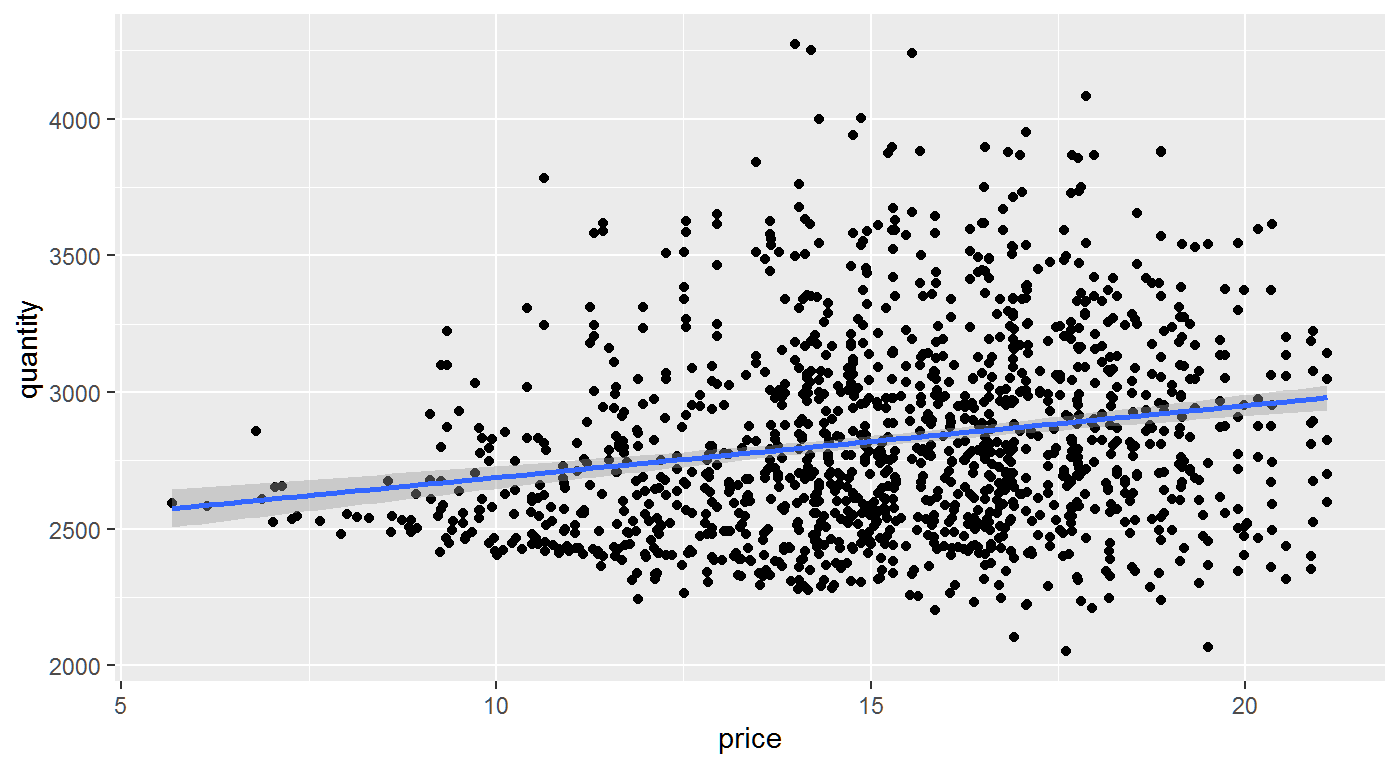
Based on this plot, it appears higher prices are associated with greater quantities sold. Should management consider raising prices? Based on this plot, it doesn’t look like higher prices would cause reduced sales.

However, if we look at individual locations, we see something quite different.

combined_df %>%
  ggplot(aes(price, quantity)) +
  geom_point() +
  geom_smooth(method = "lm") +
  facet_wrap(~ location)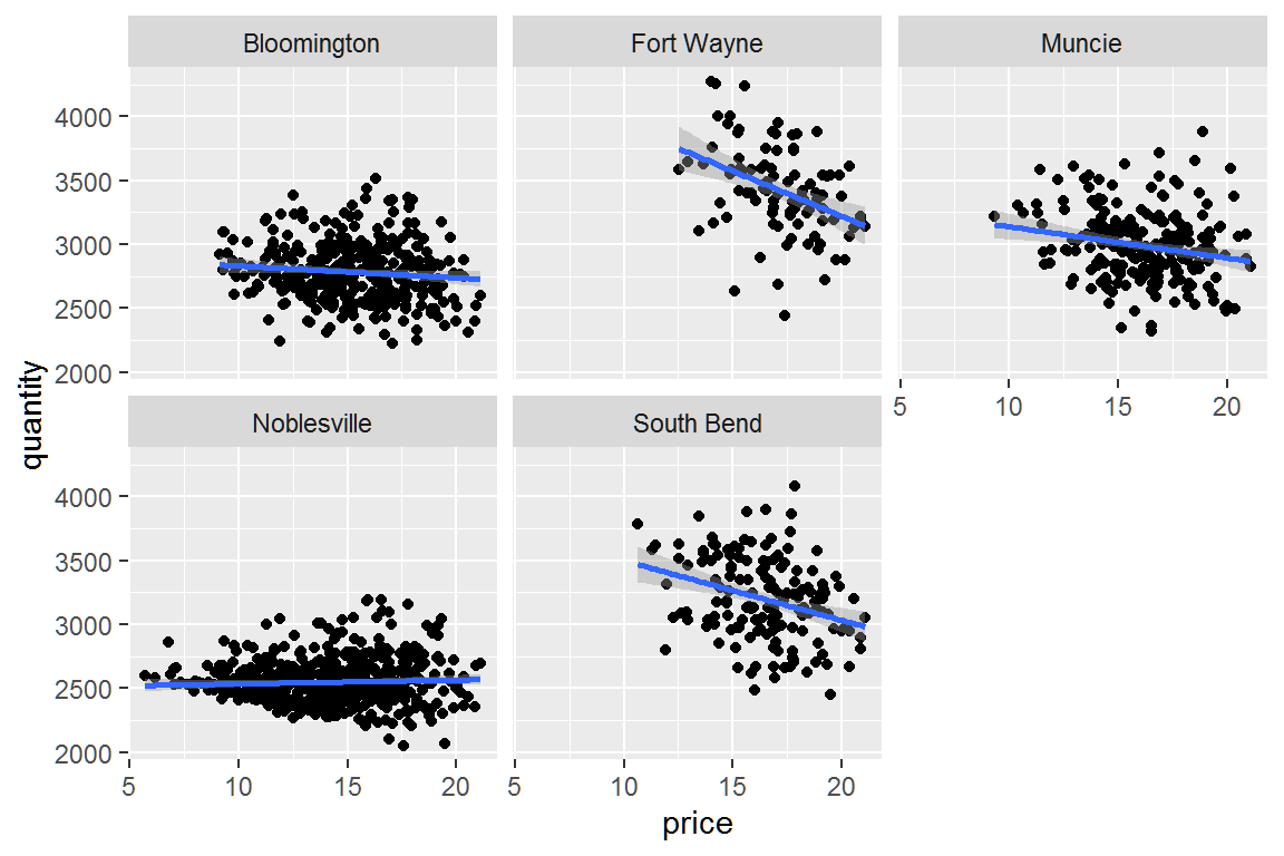

When locations are considered separately, higher prices are associated with lower quantities sold, as we would normally expect. The only exception appears to be Noblesville. Noblesville is this fictitious company’s oldest location. We have data for Noblesville from 2010 to the present.

Let’s look at Noblesville by year.

combined_df %>%
  filter(location == "Noblesville") %>%
  ggplot(aes(price, quantity)) +
  geom_point() +
  geom_smooth(method = "lm") +
  facet_wrap(~ year)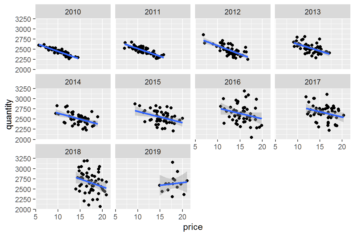

So higher prices are associated with lower quantities even for Noblesville if we look at shorter time periods like a year.

This phenomenon where an association appears to exist in data as a whole, but disappears or even reverses when groups are analyzed separately, is known as Simpson’s Paradox. You can read more about at the link.

Untidy Spreadsheet Data

David W. Body

4/16/2019