Overview of the 'pals' package
Kevin Wright
2025-03-07
Source:vignettes/pals_examples.Rmd
pals_examples.RmdThe purpose of the pals package is twofold:
- Provide a comprehensive collection of color palettes and colormaps
- Provide tools for evaluating these collections.
Memory use is reduced by compressing colormaps to fewer colors and by
calling colorRampPalette only when a colormap is
requested.
This report gives some suggestions/recommendations for color and then gives an example of each evaluation tool.
Recommendations
The appearance of color depends on:
- The display device (laptop/monitor, projector, paper, photocopy).
- The type of graphic (regions, lines).
- The person viewing the graphic (age, gender, colorblindness)
It is difficult to give definitive recommendations for the best palettes and colormaps. Nonetheless, here are some we like.
Diverging: coolwarm/warmcool (avoid Mach
banding in the middle).
Sequential (multi-hue): ocean.haline,
parula (default in Matlab).
Sequential (one hue): brewer.blues.
Rainbow: cubicl, kovesi.rainbow.
Cyclical: ocean.phase.
Categorical: brewer.paired, stepped
Bivariate: brewer.seqseq2.
## Loading required package: pals
pal.bands(coolwarm, parula, ocean.haline, brewer.blues, cubicl, kovesi.rainbow, ocean.phase, brewer.paired(12), stepped, brewer.seqseq2,
          main="Colormap suggestions")
## Only 24 colors are available with 'stepped'## Only 9 colors are available with 'brewer.seqseq2'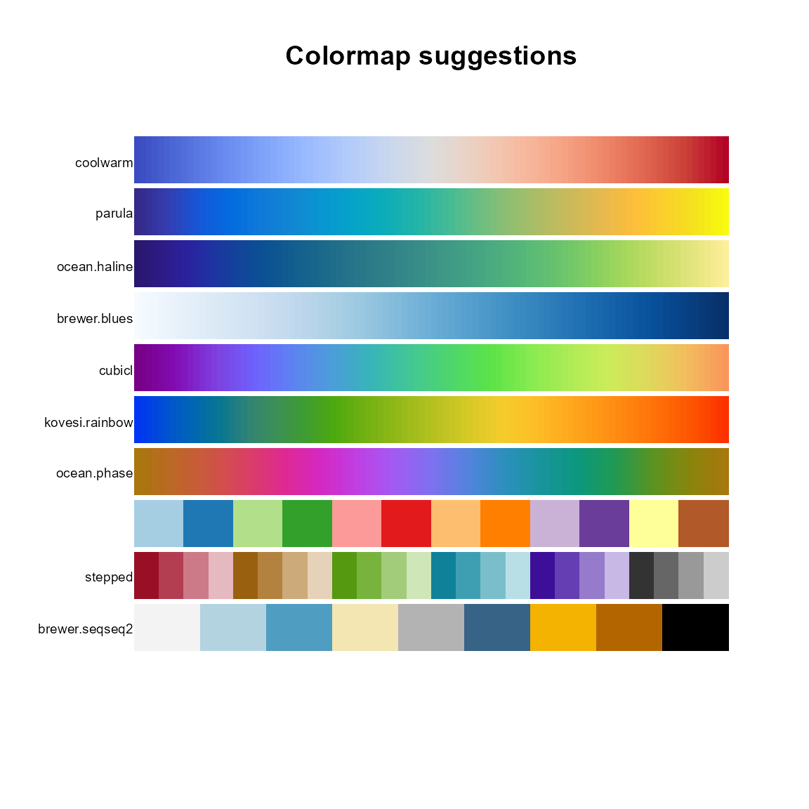
Functions in the pals package
pal.bands()
Show palettes and colormaps as colored bands
What to look for:
- A good discrete palette has distinct colors.
- A good continuous colormap does not show boundaries between colors.
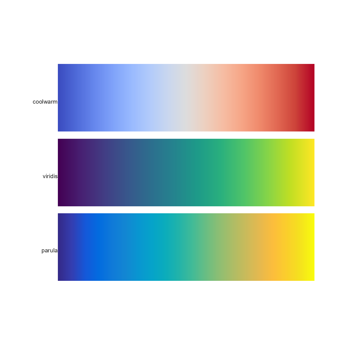
The graphic below shows what we consider to be major flaw of the viridis palette…nearly half of the palette is more or less a green color.
require(pals)
op=par(mar=c(0,5,3,1))
labs=c('alphabet','alphabet2', 'glasbey','kelly','polychrome', 'stepped', 'stepped2', 'stepped3', 'tol', 'trubetskoy','watlington')
pal.bands(alphabet(), alphabet2(), glasbey(), kelly(),
          polychrome(), stepped(), stepped2(), stepped3(),
          tol(), trubetskoy(),
          watlington(), labels=labs, show.names=FALSE)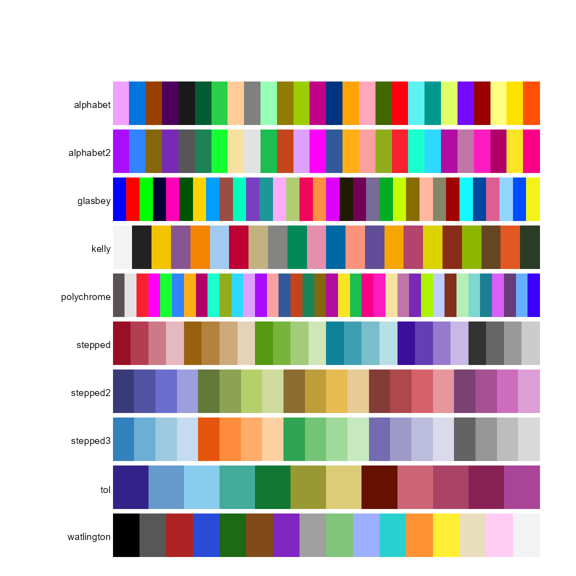
pal.channels()
Show the amount of red, green, blue, and gray in colors of a palette. The gray line corresponds to luminosity.
What to look for:
- Sequential data should usually be shown with a colormap that is smoothly increasing in lightness, as shown by the gray line.
pal.channels(parula, main="parula")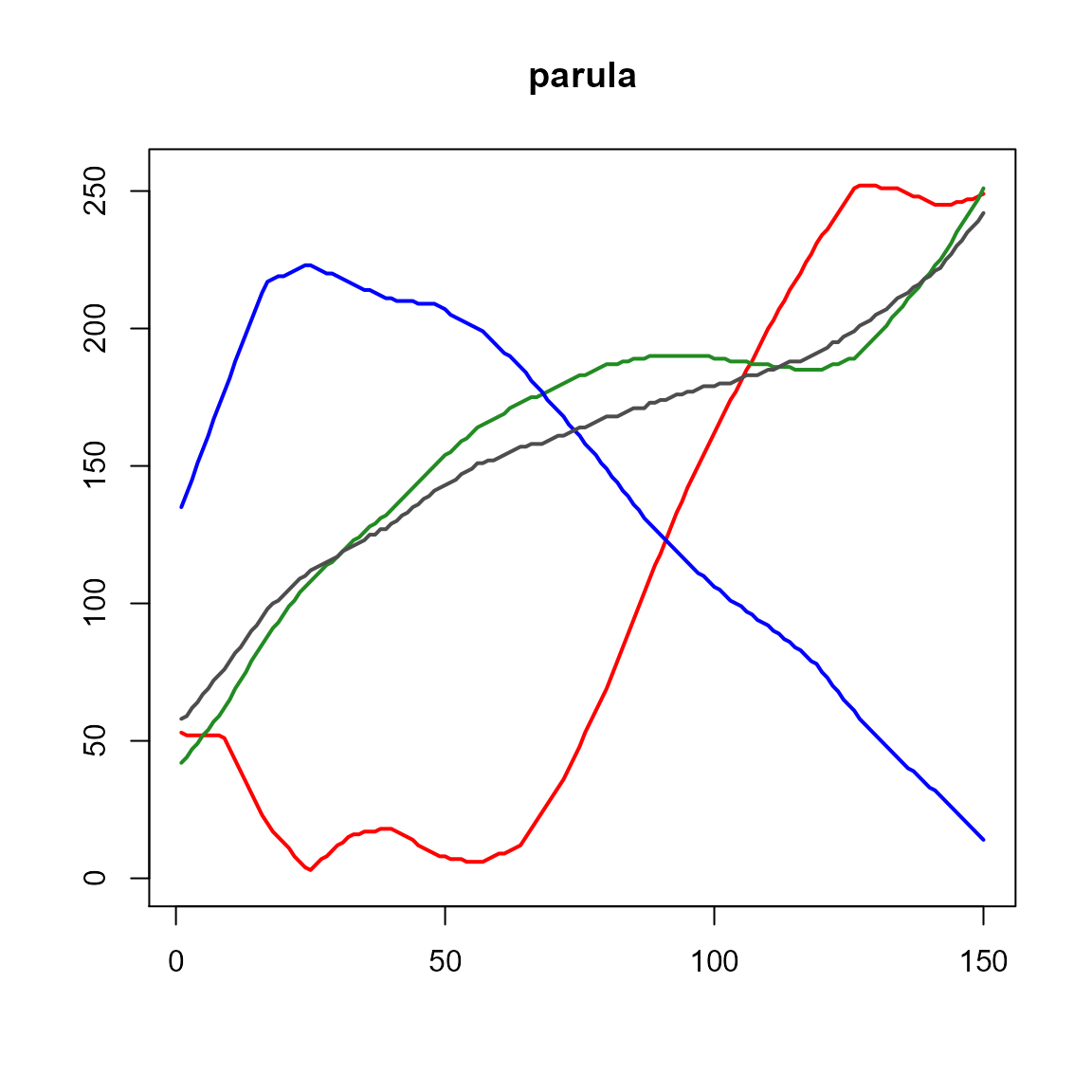
pal.cluster()
Show a palette with hierarchical clustering
The palette colors are converted to LUV coordinates before clustering.
What to look for:
- Colors that are visually similar tend to be clustered together.
- Leaves of the dendrogram should not be at substantially different heights.
pal.cluster(alphabet2(), main="alphabet2")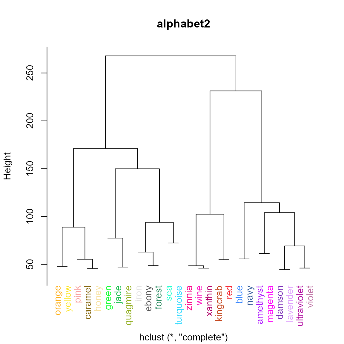
pal.compress()
A few colormaps in the pals package are defined with
mathematical formulas (e.g. the cubehelix colormap), but most of the
colormaps are originally defined as a smooth curve through a seqence of
256 colors. There seems to be no theoretical reason for 256 colors,
other than tradition. It is natural to wonder if a smooth curve through
fewer colors would be equally sufficient. This function compresses a
colormap function down to a small-ish vector of colors that can be
passed into colorRampPalette to re-create the original
palette with a non-noticeable difference. Most of the palettes in the
pals package are stored as a compressed sequence of
colors.
How effective is pal.compress? Compressing all 50
kovesi.* colormaps reduced memory from a needlessly
wasteful 352000 bytes down to 46000 bytes, a savings of 87%.
In the figure below, the top band is the (mathematically-defined)
cubehelix colormap function evaluated at 255 colors. These
256 colors are compressed to 17 colors in the cubebasis
vector (shown in the middle). These 17 colors are passed into the
colorRampPalette function and expanded to 255 colors shown
in the bottom band. The maximum squared LUV distance between the
individual colors in the two bands is only 2.34, which is smaller than
the theoretical perceptual difference of roughly 2.5.
# smooth palettes are usually easy to compress
p1 <- cubehelix(255)
cubebasis <- pal.compress(cubehelix)
p2 <- colorRampPalette(cubebasis)(255)
pal.bands(p1, cubebasis, p2,
  labels=c('cubehelix(255)', 'cubebasis','expanded'), main="compression of cubehelix")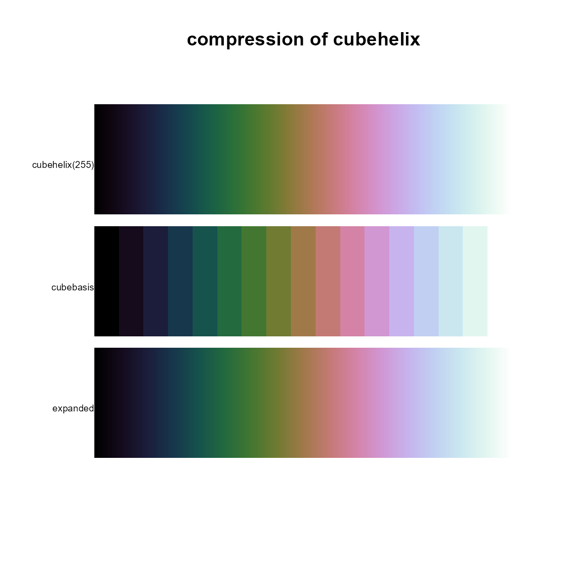
pal.maxdist(p1,p2) # 2.08## [1] 2.337919pal.csf()
Show a colormap with a Campbell-Robson Contrast Sensitivity Chart.
In a contrast sensitivity figure as drawn by this function, the spatial frequency increases from left to right and the contrast decreases from bottom to top. The bars in the figure appear taller in the middle of the image than at the edges, creating an upside-down “U” shape, which is the “contrast sensitivity function”. Your perception of this curve depends on the viewing distance.
What to look for:
- Are the vertical bands visible across the full vertical axis?
- Do the vertical bands blur together along the right side?
pal.csf(parula, main="parula")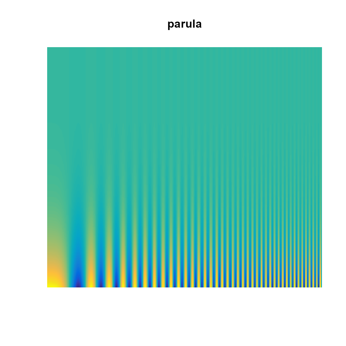
pal.cube()
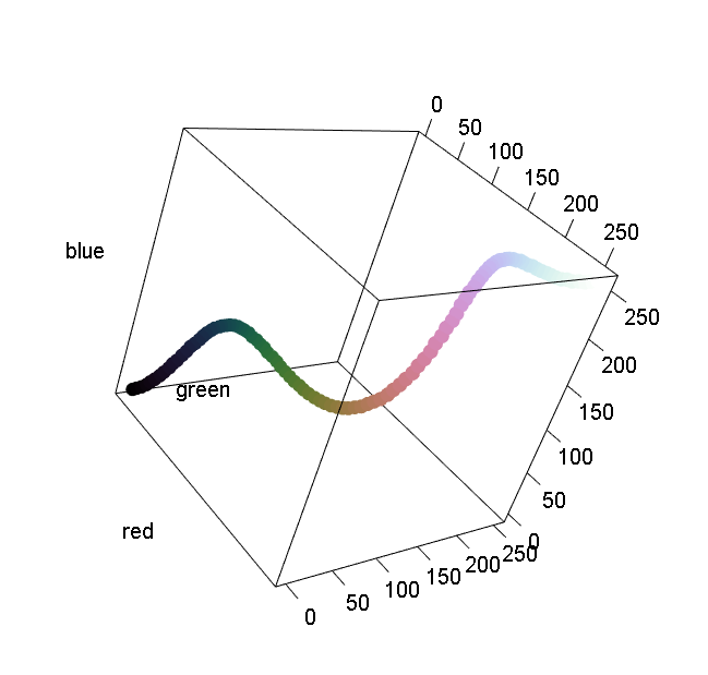
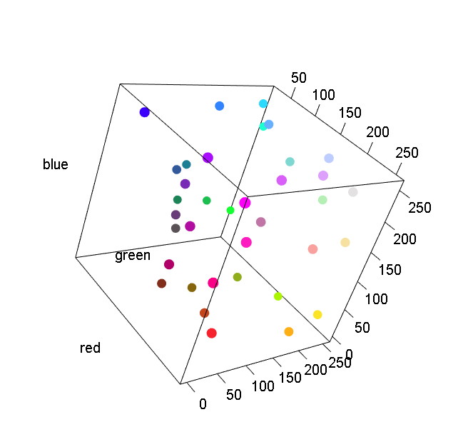
The palette is converted to RGB or LUV coordinates and plotted in a three-dimensional scatterplot. The LUV space is probably better, but it is easier to tweak colors by hand in RGB space.
pal.heatmap()
A random heatmap is generated (with 5% missing values) and a key is added to the heatmap by appending a blank column along the right side and then a column with the palette colors.
What to look for:
- Can the value of each cell be correctly inferred using the key on the right side?
- Can missing values be identified?
The graphic below shows that the alphabet2 palette is
dominated by red/pink/purple colors.
op <- par(mfrow=c(1,2), mar=c(1,1,2,2))
pal.heatmap(alphabet, n=26, main="alphabet")
pal.heatmap(alphabet2, n=26, main="alphabet2")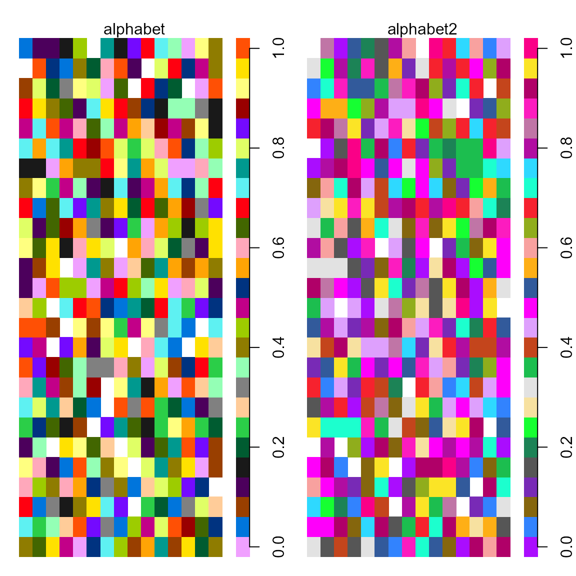
par(op)pal.heatmap2()
Display multiple palettes on a heatmap (similar to the ColorBrewer website).
What to look for:
- Are the large regions distinct from each other?
- Are rectangular outlines visible?
- Are outliers identifiable within each region?
- Are colors identifiable in the complex area (left) part of the map?
- Are missing values visible?
In the example below, the tol.groundcover palette has
several shades of green that are nearly indistinguishable.
pal.heatmap2(watlington(16), tol.groundcover(14), brewer.rdylbu(11),
  nc=6, nr=20,
  labels=c("watlington","tol.groundcover","brewer.rdylbu"))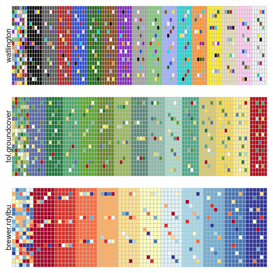
pal.map()
Display a palette on a choropleth map similar to the ColorBrewer website.
What to look for:
- Are regions distinct from each other?
- Are county outlines visible?
- Are outliers identifiable within each region?
- Are colors identifiable in the complex area (lower left) part of the map?
pal.map(brewer.paired, n=12, main="brewer.paired")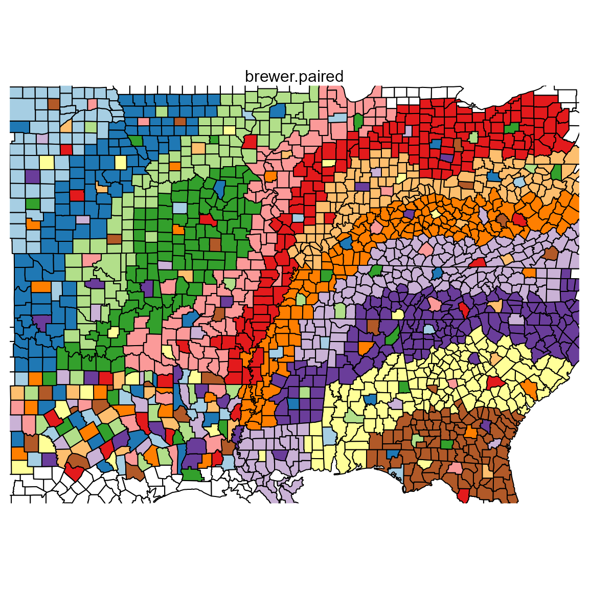
pal.safe()
A single palette/colormap is shown as five colored bands:
- Without any modifications.
- As seen in black-and-white as if photocopied.
- As seen by the deutan color-blind.
- As seen by the protan color-blind.
- As seen by the tritan color-blind.
What to look for:
- Are colors still unique when viewed in less-than full color?
- Is a sequential colormap still sequential?
pal.safe(parula, main="parula")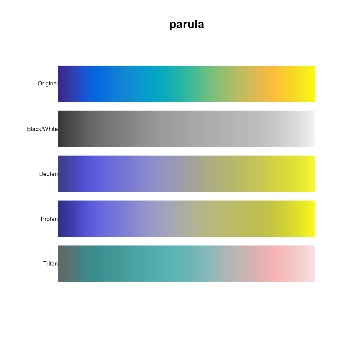
pal.scatter()
Show a colormap with a scatterplot
What to look for:
- Can the colors of each point be uniquely identified?
pal.scatter(polychrome, n=36, main="alphabet")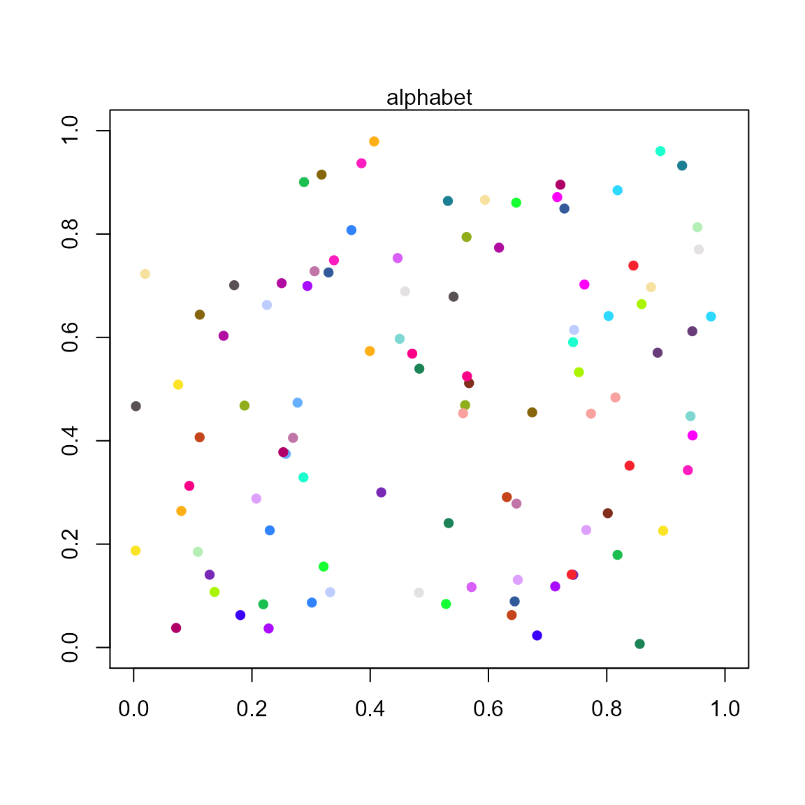
pal.sineramp()
The test image shows a sine wave superimposed on a ramp of the palette. The amplitude of the sine wave is dampened/modulated from full at the top of the image to 0 at the bottom.
What to look for:
- Along the top edge, is the sine wave equally visible across the entire image?
- Along the bottom edge, is the ramp smooth, or are there vertical bands?
pal.sineramp(parula, main="parula")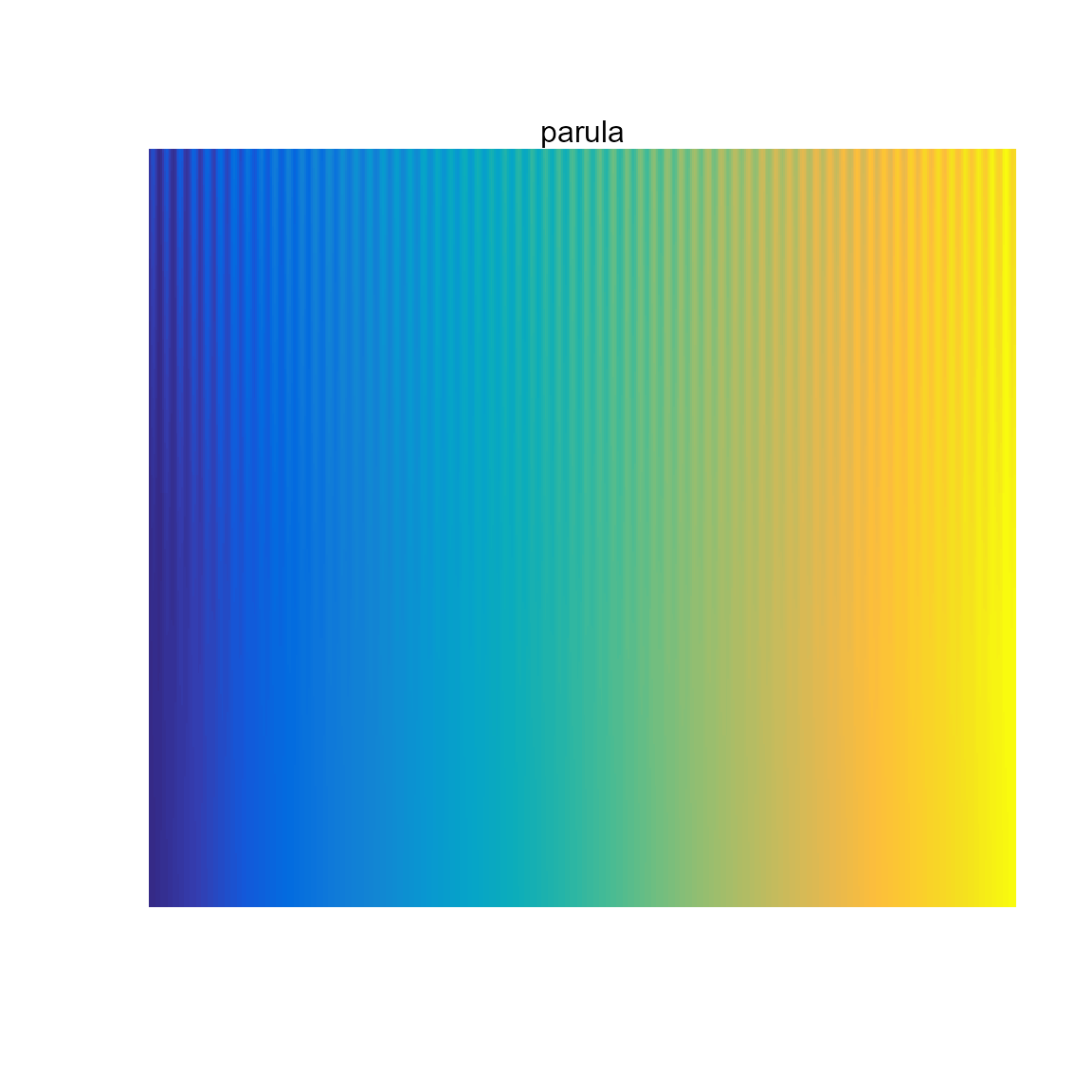
In the example below, the jet colormap fails both tests,
the tol.rainbow colormap fails to clearly show the sinewave
in the green/orange region.
op <- par(mfrow=c(3,1), mar=c(1,1,2,1))
pal.sineramp(jet, main="jet")
pal.sineramp(tol.rainbow, main="tol.rainbow")
pal.sineramp(kovesi.rainbow, main="kovesi.rainbow")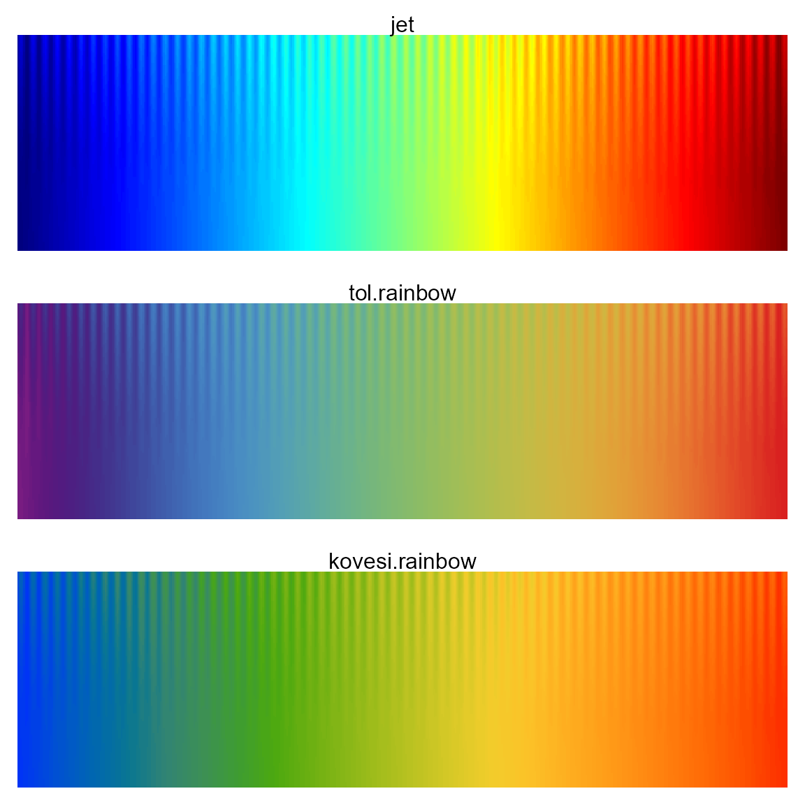
par(op)pal.test()
This function combines several other functions into a single test image.
What to look for:
- Are all squares (especially upper left and lower right) in the Z-curve distinct?
- Are the contrast sensitivity function bands visible?
- Is the sinewave showing bands of similar height, and smoothly varying along the bottom?
- Is the actual peak of the volcano identifiable? The lowest area?
- Is the gray/luminosity channel monotonic?
The examples below show the poor performance of the ‘viridis’ colormap in dark regions.
The ‘parula’ palette shows more structure in the peak of the volcano.
pal.test(parula)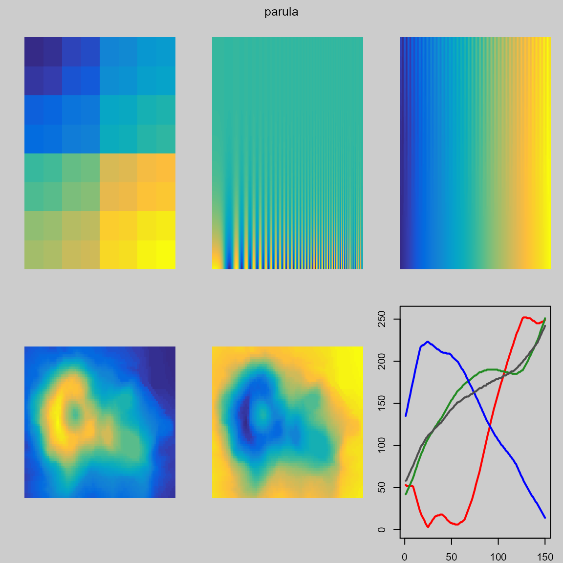
pal.test(viridis) # dark colors are poor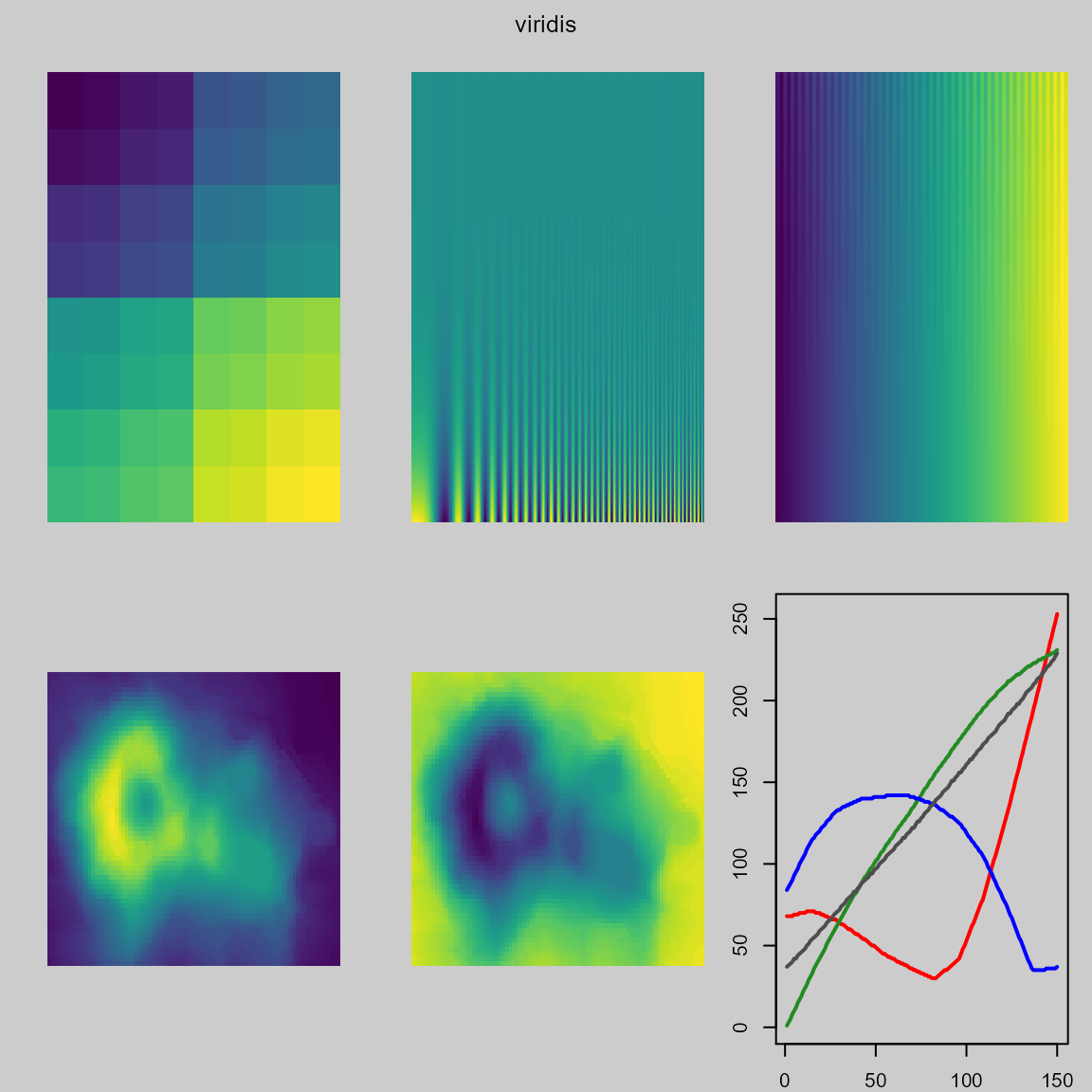
pal.volcano()
Some palettes with dark colors at one end of the palette hide the shape of the volcano in the dark colors.
What to look for:
- Can you locate the exact position of the highest point on the volcano?
- Are the upper-right and lower-right corners the same elevation?
- Do any Mach bands circle the peak?
pal.volcano(parula)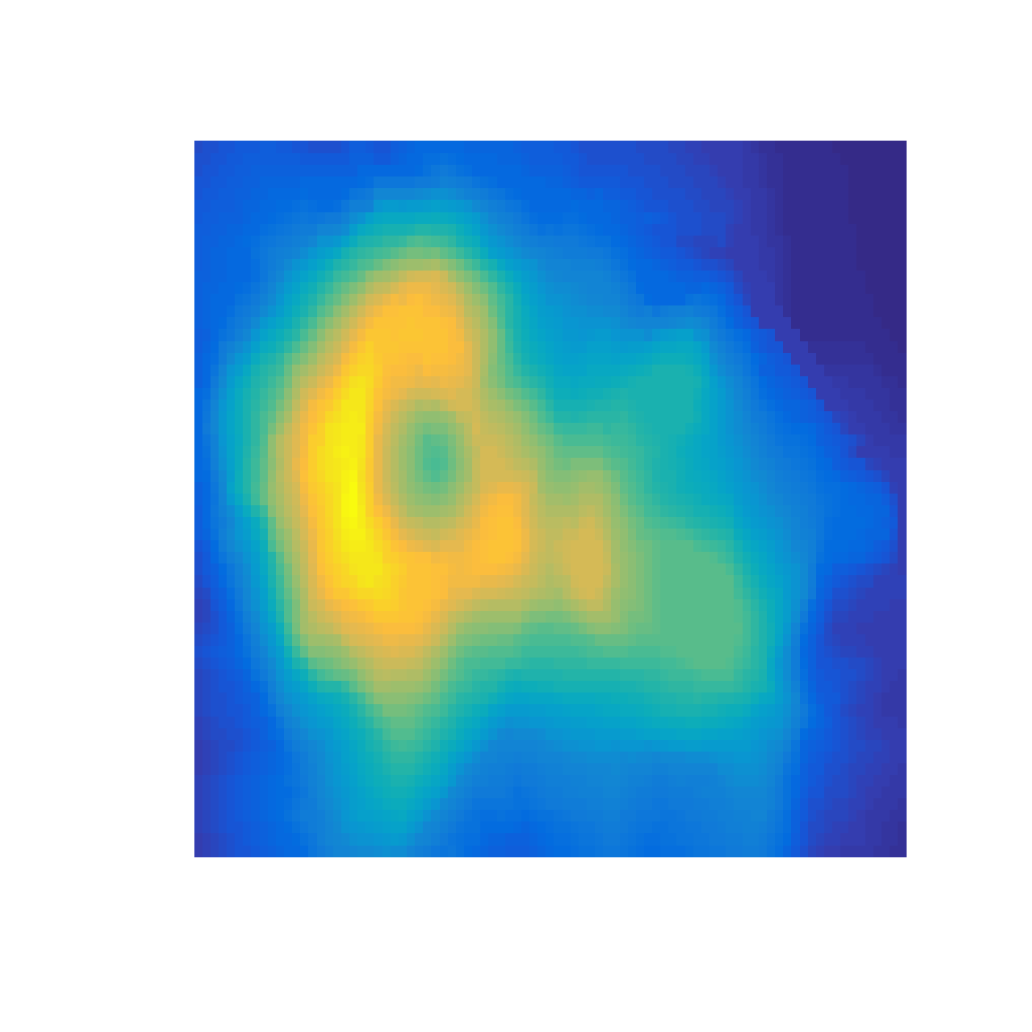
pal.volcano(viridis)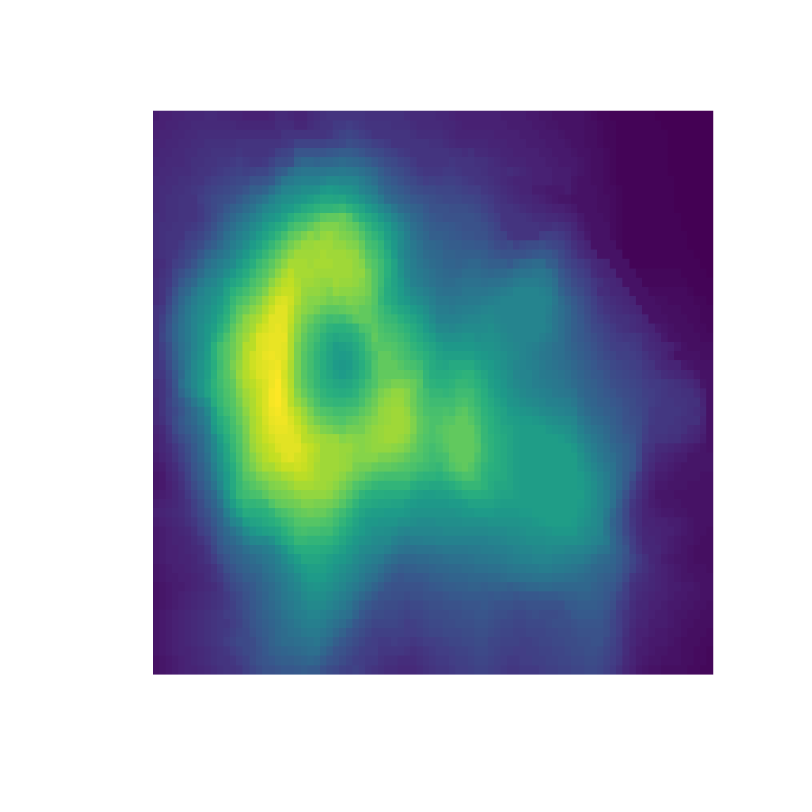
pal.zcurve()
Show a Z-order curve, coloring cells with a colormap. The difference in color between squares side-by-side is 1/48 of the full range. The difference in color between one square atop another is 1/96 the full range.
What to look for:
- A good color palette of 64 colors should be able to resolve 4 sub-squares within each of the 16 squares.
pal.zcurve(parula, main="parula")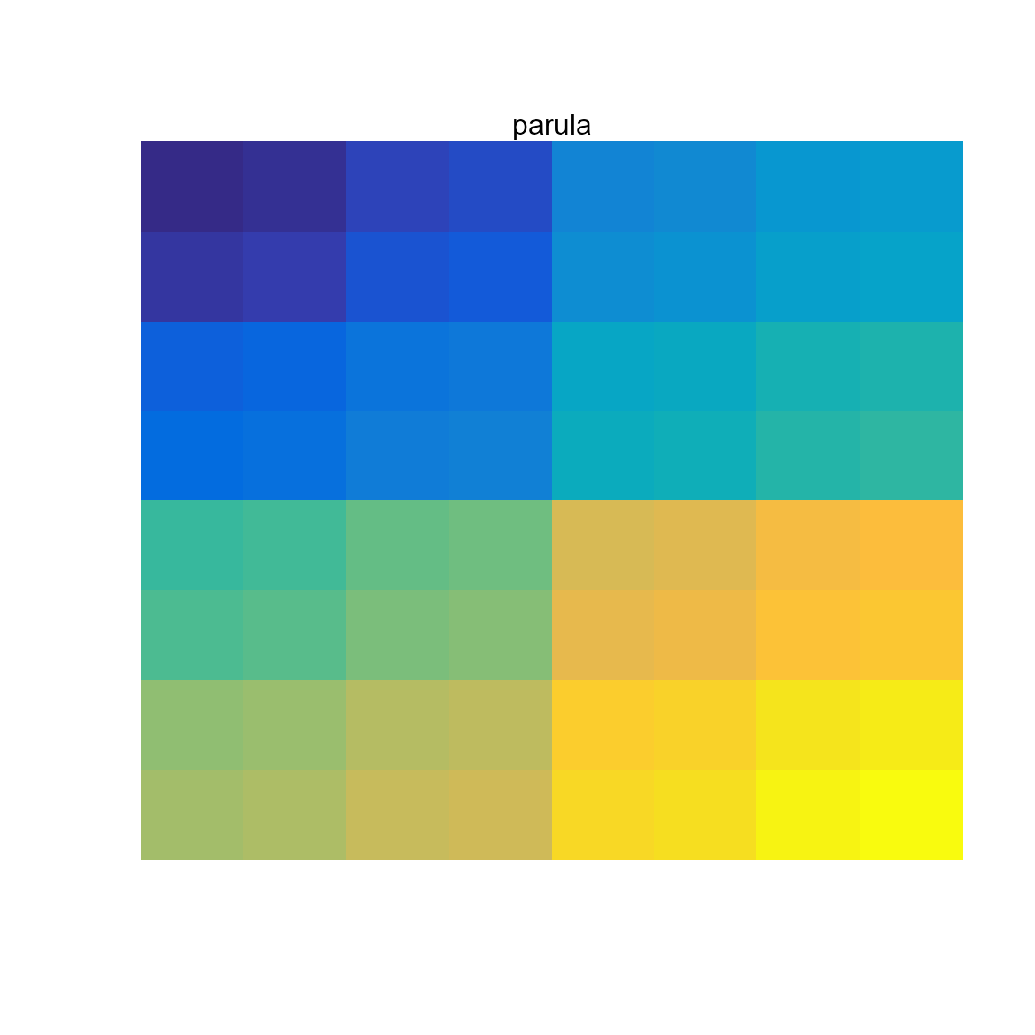
Using palettes with ggplot2
To use any colormap with the ggplot2 package, use the
ggplot2::scale_fill_gradientn() function.
## Loading required package: ggplot2## Loading required package: reshape2
ggplot(melt(volcano), aes(x=Var1, y=Var2, fill=value)) +
  geom_tile() +
  scale_fill_gradientn(colours=coolwarm(100), guide = "colourbar")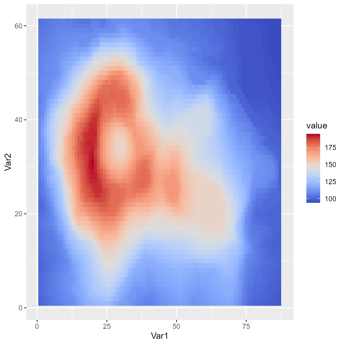
Catalog of colormaps and palettes
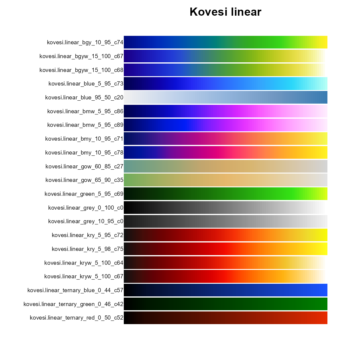
The following images show bands for all the colormaps and palettes in
the pals package, grouped in
# Discrete
pal.bands(alphabet, alphabet2, cols25, glasbey, kelly, okabe, polychrome, stepped, stepped2, stepped3, tol, watlington,
          main="Discrete", show.names=FALSE)
## Only 26 colors are available with 'alphabet'## Only 26 colors are available with 'alphabet2'## Only 25 colors are available with 'cols25'.## Only 32 colors are available with 'glasbey'.## Only 22 colors are available with 'kelly'.## Only 8 colors are available with 'okabe'.## Only 36 colors are available with 'polychrome'.## Only 24 colors are available with 'stepped'## Only 20 colors are available with 'stepped2'.## Only 20 colors are available with 'stepped3'.## Only 12 colors are available with 'tol'## Only 16 colors are available with 'watlington'.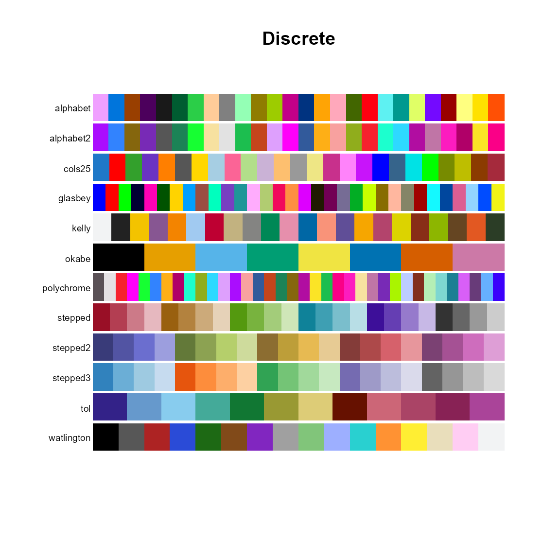
# Misc
pal.bands(coolwarm,warmcool,cubehelix,gnuplot,jet,parula,tol.rainbow,cividis)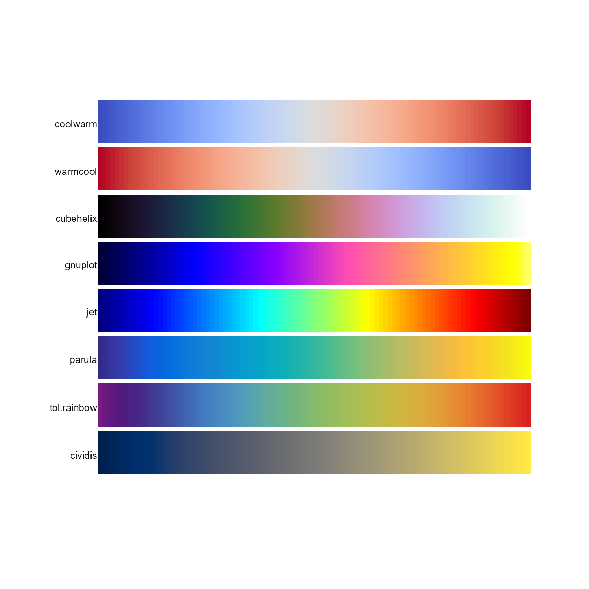
# Niccoli
pal.bands(cubicyf,cubicl,isol,linearl,linearlhot,
          main="Niccoli")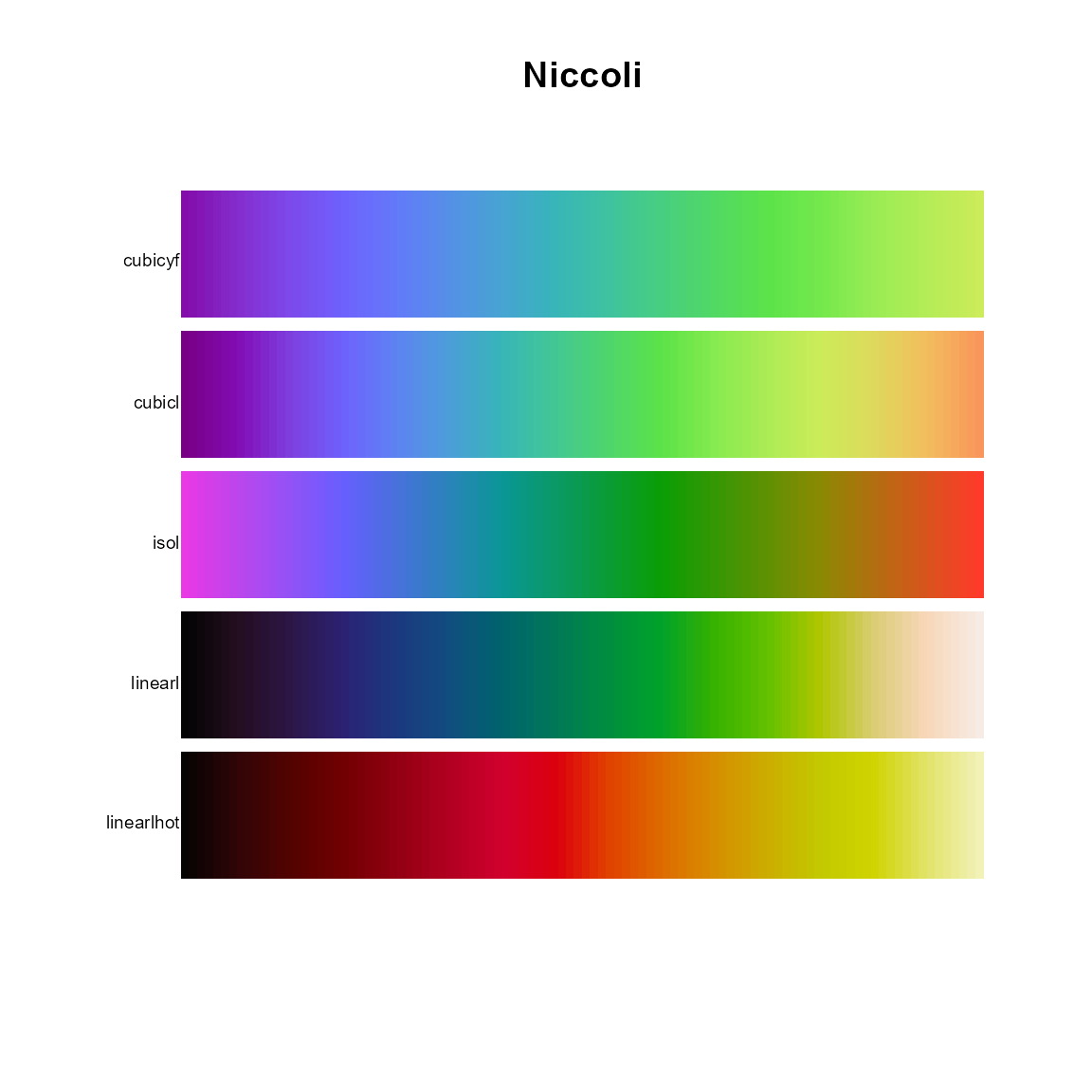
# Qualtitative
pal.bands(brewer.accent(8), brewer.dark2(8), brewer.paired(12), brewer.pastel1(9),
          brewer.pastel2(8), brewer.set1(9), brewer.set2(8), brewer.set3(10),
          labels=c("brewer.accent", "brewer.dark2", "brewer.paired", "brewer.pastel1",
                   "brewer.pastel2", "brewer.set1", "brewer.set2", "brewer.set3"),
          main="Brewer qualitative")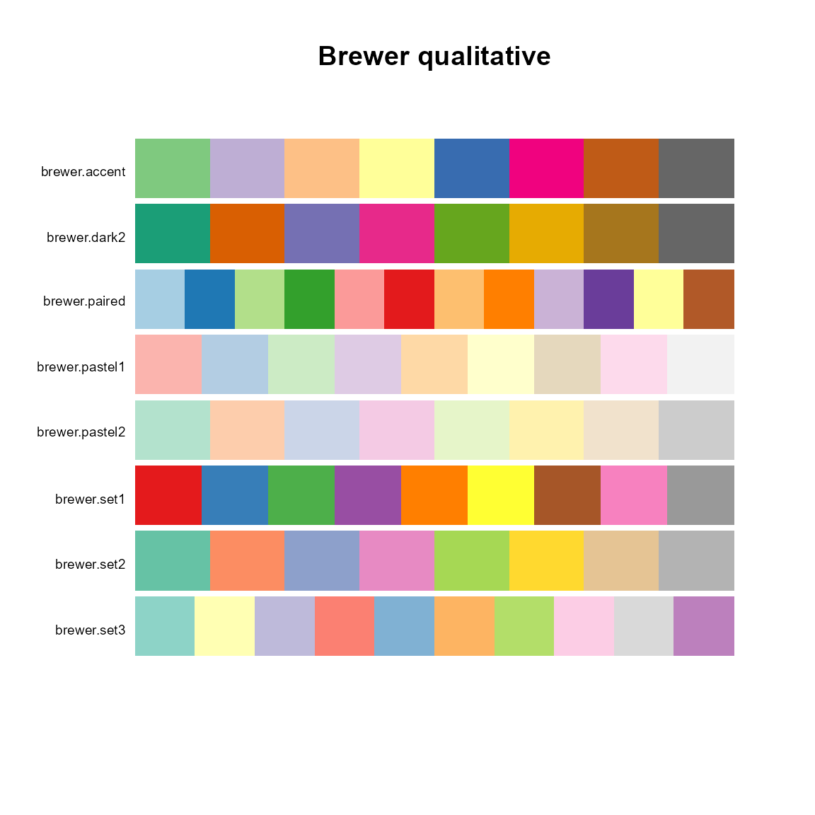
# Sequential
pal.bands(brewer.blues, brewer.bugn, brewer.bupu, brewer.gnbu, brewer.greens,
          brewer.greys, brewer.oranges, brewer.orrd, brewer.pubu, brewer.pubugn,
          brewer.purd, brewer.purples, brewer.rdpu, brewer.reds, brewer.ylgn,
          brewer.ylgnbu, brewer.ylorbr, brewer.ylorrd,
          main="Brewer sequential")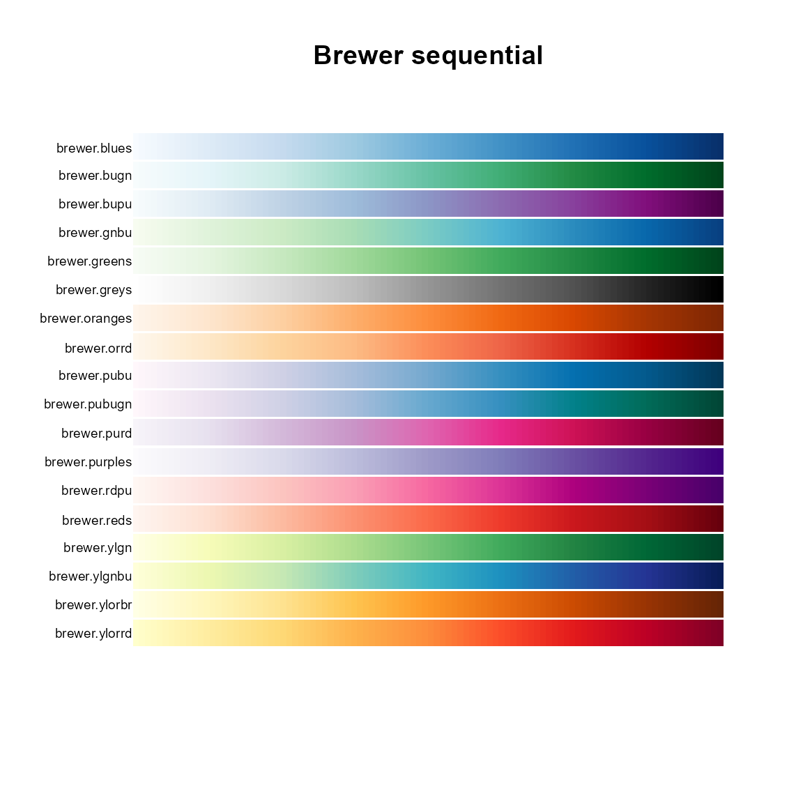
# Diverging
pal.bands(brewer.brbg, brewer.piyg, brewer.prgn, brewer.puor, brewer.rdbu,
          brewer.rdgy, brewer.rdylbu, brewer.rdylgn, brewer.spectral,
          main="Brewer diverging")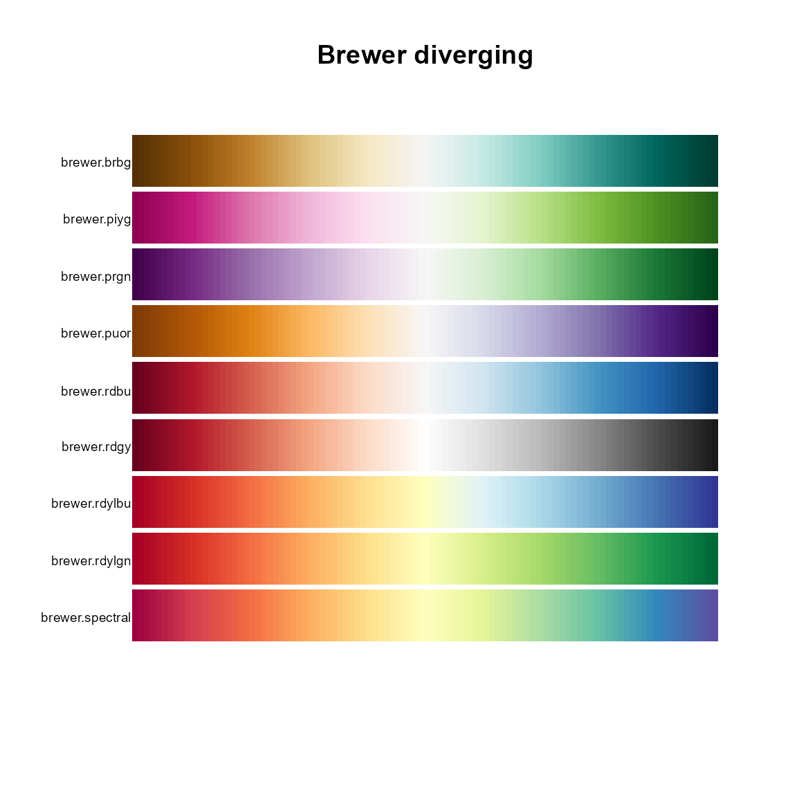
# Ocean
pal.bands(ocean.thermal, ocean.haline, ocean.solar, ocean.ice, ocean.gray,
          ocean.oxy, ocean.deep, ocean.dense, ocean.algae, ocean.matter,
          ocean.turbid, ocean.speed, ocean.amp, ocean.tempo, ocean.phase,
          ocean.balance, ocean.delta, ocean.curl, main="Ocean")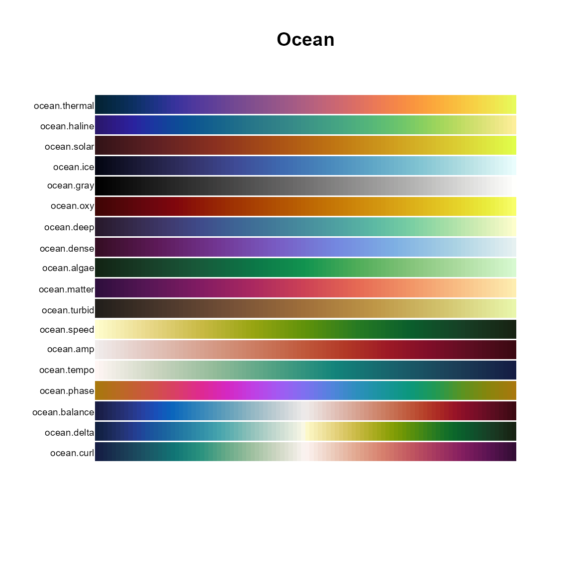
# Matplotlib
pal.bands(magma, inferno, plasma, viridis, main="Matplotlib")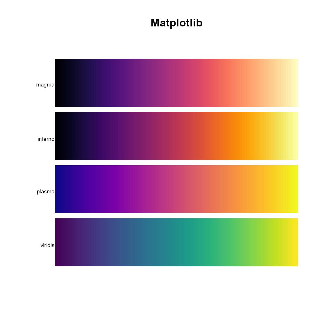
# Kovesi
op = par(mar=c(1,10,2,1))
pal.bands(kovesi.cyclic_grey_15_85_c0, kovesi.cyclic_grey_15_85_c0_s25,
kovesi.cyclic_mrybm_35_75_c68, kovesi.cyclic_mrybm_35_75_c68_s25,
kovesi.cyclic_mygbm_30_95_c78, kovesi.cyclic_mygbm_30_95_c78_s25,
kovesi.cyclic_wrwbw_40_90_c42, kovesi.cyclic_wrwbw_40_90_c42_s25,
kovesi.diverging_isoluminant_cjm_75_c23, kovesi.diverging_isoluminant_cjm_75_c24,
kovesi.diverging_isoluminant_cjo_70_c25, kovesi.diverging_linear_bjr_30_55_c53,
kovesi.diverging_linear_bjy_30_90_c45, kovesi.diverging_rainbow_bgymr_45_85_c67,
kovesi.diverging_bkr_55_10_c35, kovesi.diverging_bky_60_10_c30,
kovesi.diverging_bwr_40_95_c42, kovesi.diverging_bwr_55_98_c37,
kovesi.diverging_cwm_80_100_c22, kovesi.diverging_gkr_60_10_c40,
kovesi.diverging_gwr_55_95_c38, kovesi.diverging_gwv_55_95_c39,
kovesi.isoluminant_cgo_70_c39, kovesi.isoluminant_cgo_80_c38,
kovesi.isoluminant_cm_70_c39, kovesi.rainbow_bgyr_35_85_c72, kovesi.rainbow_bgyr_35_85_c73,
kovesi.rainbow_bgyrm_35_85_c69, kovesi.rainbow_bgyrm_35_85_c71,
main="Kovesi")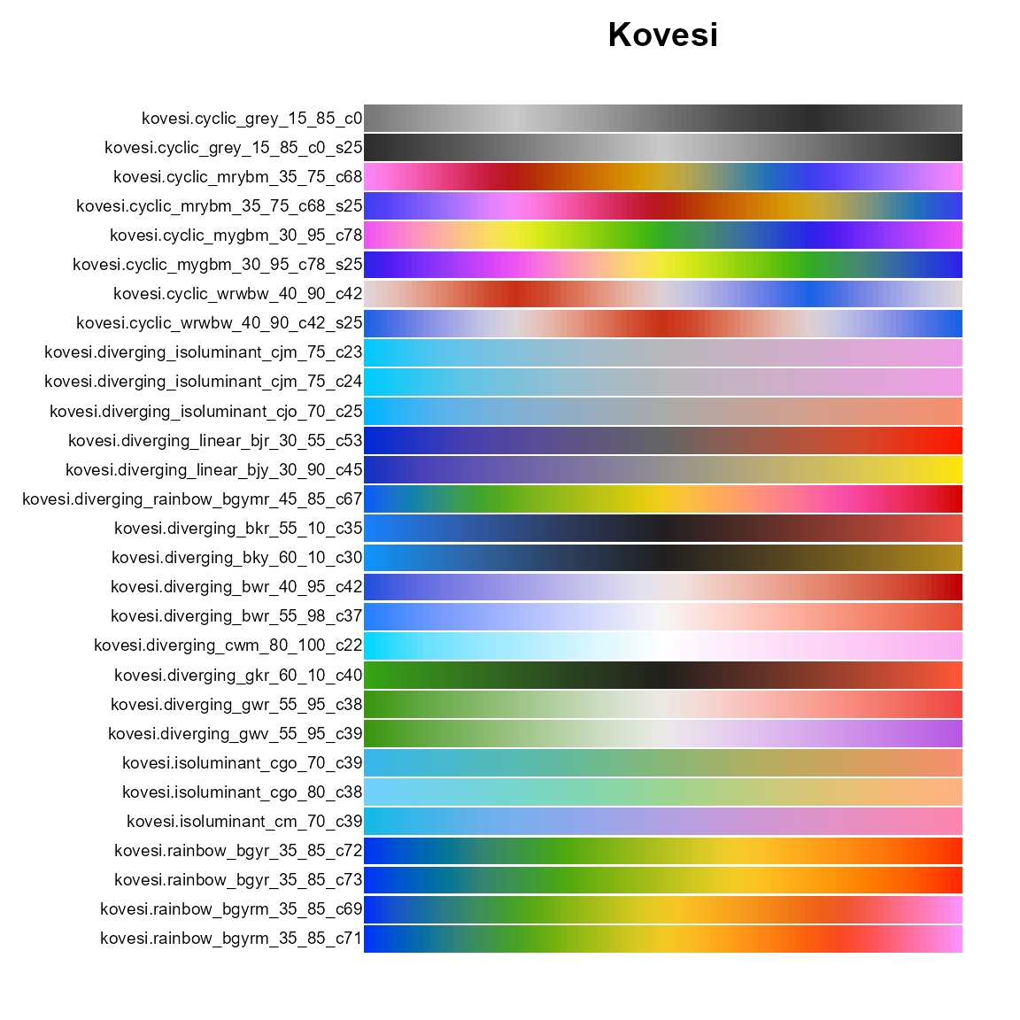
pal.bands(kovesi.linear_bgy_10_95_c74,
kovesi.linear_bgyw_15_100_c67, kovesi.linear_bgyw_15_100_c68,
kovesi.linear_blue_5_95_c73, kovesi.linear_blue_95_50_c20,
kovesi.linear_bmw_5_95_c86, kovesi.linear_bmw_5_95_c89,
kovesi.linear_bmy_10_95_c71, kovesi.linear_bmy_10_95_c78,
kovesi.linear_gow_60_85_c27, kovesi.linear_gow_65_90_c35,
kovesi.linear_green_5_95_c69, kovesi.linear_grey_0_100_c0,
kovesi.linear_grey_10_95_c0, kovesi.linear_kry_5_95_c72,
kovesi.linear_kry_5_98_c75, kovesi.linear_kryw_5_100_c64,
kovesi.linear_kryw_5_100_c67, kovesi.linear_ternary_blue_0_44_c57,
kovesi.linear_ternary_green_0_46_c42, kovesi.linear_ternary_red_0_50_c52,
main="Kovesi linear"
)
par(op)


# Bivariate
bivcol <- function(pal, nx=3, ny=3){
  tit <- substitute(pal)
  if(is.function(pal)) pal <- pal()
  ncol <- length(pal)
  if(missing(nx)) nx <- sqrt(ncol)
  if(missing(ny)) ny <- nx
  image(matrix(1:ncol, nrow=ny), axes=FALSE, col=pal)
  mtext(tit)
}

op <- par(mfrow=c(4,4), mar=c(1,1,2,1))
bivcol(arc.bluepink)
bivcol(brewer.divbin, nx=3)
bivcol(brewer.divdiv)
bivcol(brewer.divseq)
bivcol(brewer.qualbin, nx=3)
bivcol(brewer.qualseq)
bivcol(brewer.seqseq1)
bivcol(brewer.seqseq2)
bivcol(census.blueyellow)
bivcol(stevens.bluered)
bivcol(stevens.greenblue)
bivcol(stevens.pinkblue)
bivcol(stevens.pinkgreen)
bivcol(stevens.purplegold)
bivcol(tolochko.redblue)
bivcol(vsup.redblue, nx=8)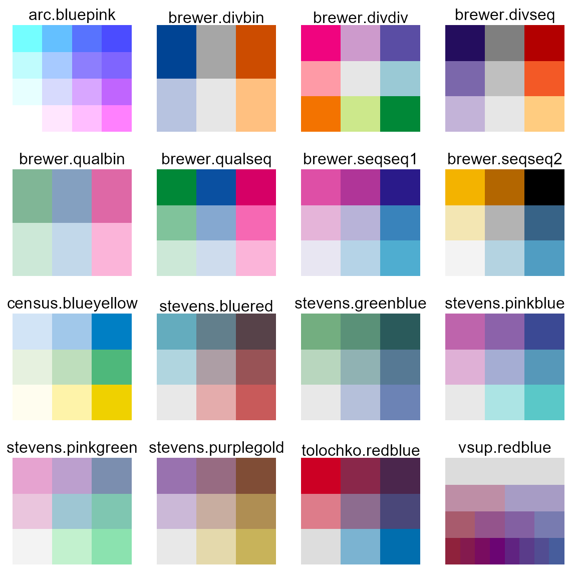
par(op)